1. Introduction
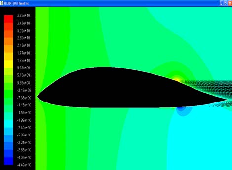
marine propeller is a propulsion system which turns the power delivered by the engine into thrust to drive the vessel through water. Propeller cavitation is a general problem encountered by the ship owner, whereby it causes vibrations, noises, degradation of propeller performance, deceases engine efficiencies, effects the life cycle of the ship and also results in high cost of maintenance. The basic physics of cavitation occurs when the pressure of liquid is lower or equal to the vapour pressure, which depends on the temperature, thus forming cavities or bubbles. The compression of pressure surrounding the cavities would break the cavities into smaller parts and this increases the temperature. Collapse of bubbles in contact with parts of the propeller blades will create high localised forces that subsequently erode the surface of the blades. Simulation on cavitating flow using CFD can be carried out to determine the performance of the propeller. A model is generated in Gambit and fluid-flow physics are applied to predict the fluid dynamics and other physical phenomena related to thepropeller. Ref. [1] stated that, CFD can provide potential flow analysis such as flow velocities and pressure at every point in the problem domain as well as the inclusion of viscous effects. a) Previous studies on propeller cavitation Ref. [2] in their studies, generated hybrid grid of about 187 000 cells using Gambit and T Grid. The blade surface was firstly meshed with triangles including the root, tip and blade edges. The turbulent boundary layer was resolved with four layers of prismatic cells between blade and hub surfaces. In the cavitating propeller case, the boundary conditions were set to simulate the flow around a rotating propeller in open water. Inlet boundary, velocity components for uniform stream, blade and hub surfaces, and outer boundary were included. This ensured the rotational periodicity of the propeller on the exit boundary by setting the pressure corresponding to the given cavitation number and other variables was later extrapolated [3,11]. On the other hand, [3] applied a mixture of models with algebraic slip to simulate cavitating flow over a NACA 66 hydrofoil. This multiphase flow model which used incompressible fluids consisting of liquid and vapour was used as primary and secondary phase respectively. Structured quadrilateral grids of 19 490 cells were meshed. Inflow and outflow boundary were indicated as velocity magnitude and direction and zero gauge pressure respectively. Contour of vapour volume fraction shown in Figure 1 indicates that cavity can be observed at the mid-chord region [4,12]. This study is focussed mainly on simulating a cavitating flow at the propeller blade section of Kaplan series in order to optimize the propeller blade to increase its performance. Two-dimensional simulations of different radii were carried out at different revolutions per minute (rpm) and the results were compared based on the pressure difference. The objective is to simulate and investigate the water flow at the propeller blade A section and to recommend measures to reduce cavitation in order to increase its efficiencies [4,5].
2. II.
3. Methodology a) Model generation in Gambit
The Propeller Blade models of 0.2R and 0.6R were generated and computational domains were created to assume water is flowing from far towards the Propeller Blade. Figure 2 and Table 1 show far-field boundary conditions surrounding the Propeller Blade. Then, meshing was carried out between the boundaries and Propeller Blade to determine the accuracy of the model generation. Figure 3 and 4 show the meshing process [6,13,14]. Propeller blades of 0.2R and 0.6R were simulated in Fluent 6.3.26. Pressure-based numerical solver, laminar and turbulent physical model were selected as the functioning base for 300rpm and 600rpm. Then, the material properties, for instance, the density of sea water and viscosity value were defined and calculated based on Table 2.. Consequently, the operating condition was set to be 2296 Pa, which is the condition for vapour pressure at sea water when the temperature is 20°C. On the other hand, the boundary conditions of far field 1 and far field 2 were specified as velocity inlet, whereby the velocity magnitude and direction were calculated [7,8].
As for far field 3, this boundary was specified as pressure outlet; the gauge pressure was set to be 0 Pa. The existence of inflow and outflow boundaries enables the characteristics of fluid to be observed by entering and leaving the flow domain. The turbulent viscosity ratio was set to correspond to the default value for 600rpm of both radii. Next, the solution procedure was set as simple algorithm, and under discretisation, the pressure and momentum were set as Standard and First Order Upwind respectively [9,10].
4. Dynamic viscosity = kinematic viscosity x density (1)
Therefore, the calculated dynamic viscosity is 1.08035 x 10 9 kg/m.s.
Consequently, the operating condition was set to be 2296 Pa based on Table 3, which is the condition for vapour pressure at sea water when the temperature is 20°C. On the other hand, the boundary conditions of far field 1, far field 2 and far field 3 were specified to accommodate the fluid behaviour. Far field 1 and far field 2 were specified as velocity-inlet, whereby the velocity magnitude and direction were calculated as the following:
For 0.2R airfoil section profile, Pitch angle, ? = tan -1 ( P 2?r ), (2) where, P is pitch and r is radius of the blade section Thus, resultant velocity of the fluid flow at 0.2R is calculated as,
Resultant velocity, v = ( 2?rn cos ? ),(3)Where, n is equal to the rotational speed of the propeller
Resultant velocity, v = ( 2?rn cos ? ),(4)Velocity-inlets at both far fields were then indicated as 729 m/s for 0.2R airfoil section. As for far field 3, this boundary was specified as pressure-outlet, whereby the gauge pressure was set to be zero Pascal. The existence of inflow and outflow boundaries enables the characteristics of fluid to be observed by entering and leaving the flow domain. Parameters in the solution control were set up to select the suitable iterative solvers. Under pressure-velocity coupling, the solution procedure was set as SIMPLE algorithm, which equipped an accurate linkage between pressure and velocity. SIMPLE algorithm was used due to the assumption of steady flows. Besides, under discretization, the pressure and momentum were set as Standard and First Order Upwind respectively. The First Order Upwind was set due to convection terms in solution, thus the face value would be set to cell-centre value. This was done before any CFD calculation was performed. The solution was then initialised and computed from far field 1.
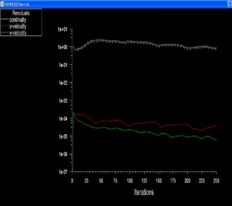
Monitoring of the convergence of the solution was performed. There were three differential equations to be solved in a two-dimensional incompressible laminar flow problem, which indicated the three residuals to be monitored for convergence, that is, continuity, x-velocity and y-velocity. The default convergence criteria were set as 0.001 for all three of these. As the code iterates, the residuals were calculated for each flow of equation. These residuals represented an average error in the solution. Moreover, monitoring lift and drag force was carried out and calculated as following: For 0.2R airfoil section profile,
Angle of attack, ? = ( 2fmax C ) (5)Where, f max is thickness of the airfoil section and C is chord length of the airfoil section Angle of attack, ? = ( 2fmax C ) (6) Lift force is defined as a force perpendicular to the direction of the freestream. Therefore, X and Y are formulated as sin ? and negative cos ?, respectively, as shown in Figure 5. As for the drag force vector, it is defined as the force component in the direction of the freestream.
Thus, X and Y are formulated as negative cos ? and sin ? respectively, as shown in Figure 6. Therefore, lift force vectors at X and Y were -0.5736 and 0.819 respectively.
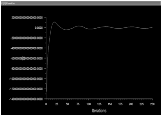
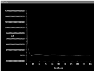
The solution was solved and iterated in order to remove the unwanted accumulations, so that the iterative process would converge rather than diverge. A converge solution is usually achieved when the residuals fall below some convergence criteria, that is 0.001. Besides examining residuals, variables such as lift and drag force were monitored to find out the convergence of the numerical computations.
Last but not least, the CFD results were visualised and analysed at the end of the computational simulation in different categories, such as vector plots and contour plots for a better relevant physical characteristics view within the fluid -flow problem.
The simulation process was repeated by inserting various operating pressure values below 2296 Pa in order to observe the pressure difference for cavitation to occur and also to examine the sensitivity for accuracy of the results and performance. Finally, document the findings of the analysis.
5. III.
6. Results and Discussions
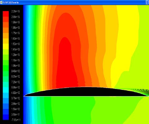
Three Propeller Blade section profiles at different radii, such as 0.2R, 0.6R and 1.0R were simulated. The CFD results were then visualised and analysed for comparison. 6, it can be seen that the residuals were moving upwards and not fulfilling the converging criteria, that is to be below 0.001. This shows that the solution was diverging instead of converging. As for the lift and drag vector force, Figure 8 and 9 shows a divergence result which is not compatible with the convergence criteria. For 0.6R Propeller Blade section, the CFD results, for instance, three residuals of CFD calculation, lift and drag force, velocity vector plot, and contour plot were visualised and analysed (Figure 11). f) Iteration of 0.6R Figure 14 shows 250 iteration results, whereby the continuity, x-velocity and y-velocity were calculated for flow equation. It can be seen that the residuals were moving downwards equivalent to the convergence criteria, which is 0.001. This shows that the solution was converging. Based on the above contours, cavitations can happen if the Propeller Blade radius section increases, especially for 0.6R compared to 0.2R. This is because the bigger the radius, themore pressure would be concentrated at that location. Besides this, in the turbulent flow, cavitation is more likely to be induce compared to laminar flow due to its fluid characteristics. Also, the higher the rpm, the lower the absolute pressure.
7. g) Graph of absolute pressure versus curve length
The graph in Figure 19 shows that, the pressure decreases when it passes by the Propeller Blade equivalent to the diagrams shown above and as it leaves the Propeller Blade, the pressure slowly increases back to its actual pressure. Figure 20 shows cavitation number, ? versus advance coefficient, based on the graph. When the propeller rotates at 300rpm, the operating condition falls in the region for a conventional propeller, which is suitable for most of the merchant vessels, whereas, at 600rpm, propeller operating condition falls in the poor region for high -speed propeller operation. This indicates low efficiency for propeller since low advance coefficient implies high propeller power coefficient. This is probably due to inaccurate application of propeller rotational speed with engine load and gear box used.
When the propeller rotates at 300rpm, the advance coefficient and cavitation number reaches the region for conventional propeller operation. This means that, at 300rpm, the propeller rotates at a good condition suitable to the engine load and gear box required. On the other hand, when the propeller rotates at higher speed, it reaches a poor region for highspeed propeller operation which indicates damages, vibration and cavitation would occur. Based on the results of velocity and contour plots of 300rpm and 600rpm, the higher the rpm, the lower the absolute pressure, which is the condition for cavitation to occur. This is caused by high rotational rates of the propeller which creates high -pressure and low-pressure region on the blades. Besides, when the radius increases along the propeller, cavitation might happen too. Airfoil section profile at 0.2R does not have cavitation due to less pressure concentration in that region compared to 0.6R airfoil section profile. At 0.6R airfoil section profile, more works is required to be done in that region [14,15].
8. IV.
9. Conclusion
The paper presents the result of water flow at the blade section profile. Cavitation occurrence is observed to be at the upper surface of 0.6R compared to 0.2R of propeller blade section due to different pressure concentrations. Besides, cavitation is predicted at low absolute pressure when the rpm is high and this correlates with theory hypothesis. Optimisation of the propeller can be achieved by increasing the blade area ratio (BAR) and compare it with the standard Kaplan BAR value that is, 0.85. The result deduced from this study can be added to existing databased for validation purposes especially for ship navigating within Malaysian water. This could provide information on environmental differential impact on propeller. It is recommended that further multiphase, experimental simulation should carried out to test rotational speed of propeller at different powers produced by the engine load.
V.

| Temperature | Density | Kinematic | ||
| (°C) | (kg/ m 3 ) | viscosity | ||
| (m 2 /s x 10 6 ) | ||||
| Fresh | Salt | Fresh | Salt | |
| water | water | water | water | |
| 0 | 999.8 | 1028.0 | 1.787 | 1.828 |
| 10 | 999.6 | 1026.9 | 1.306 | 1.354 |
| 20 | 998.1 | 1024.7 | 1.004 | 1.054 |
| 30 | 995.6 | 1021.7 | 0.801 | 0.849 |
| sea water (Carlton, 2007) | ||||||
| Temperatur e (°C) | 0.01 5 | 10 | 15 | 20 | 25 | 30 |
| Fresh water, P v | 611 872 1228 1704 2377 3166 4241 | |||||
| (Pa) | ||||||
| Sea water, P v (Pa) | 590 842 1186 1646 2296 3058 4097 | |||||