1. Introduction
different compared with the radial system. Furthermore, protective relays on the main feeder must see fault currents in forward or reverse directions, and they have to detect the fault direction. Another important problem is that DGs can get disconnected from the grid due to disturbances or for maintenance. [1] Consequently, a new configuration for the system results and, if a fault occurs, a different fault current level flows. Therefore, one setting for the protective relays cannot adequately respond to the continuously changing system configuration. Thus, relays have to be adaptively coordinated for each new system configuration to achieve correct fault clearance operation.
2. II.
3. DG Installation Problem Formulation
In this work the objective of the placement technique for the DG is to minimize the real power loss and to improve the voltage profile at the distribution level. The real power loss reduction in a distribution system is required for efficient power system operation. The loss in the system can be calculated using (1) in [3], called the 'exact loss formula' given the system operating conditions. The objective of the placement technique is to minimize the total real power loss and improved voltage profile. Mathematically, the objective function can be written as:
???????????????? ?? ?? = ?|?? ?? | 2 ?? ??=1 ?? ??(1)Subject to power balance constraints. Where i is the number of bus, N is the total number of Buses, ?? ?? is the real power loss in the system, © 2020 Global Journals istributed Generators (DG) are increasingly connected to distribution systems to meet the load demand and increase the reliability of the system. With the additional connected sources, the system is no longer radial. Moreover, during a fault condition, the fault is fed from all the sources connected to the power system. Therefore, the fault current level is ?? ?????? is the real power generation of DG at bus i, ?? ???? is the power demand at bus i , ?? ???? is the current between buses i and j ?? ?? is the resistance.
4. ? ?? ??????
The current ?? ?? is determined from the load flow using Hybrid load flow studies Method called Backward -Forward and Newton Raphson. For single source network all the power is supplied by the source but with DG that are optimally placed there is going to be reduction in power loss. [4] This reduction in power loss is determined as the difference of the power loss with DG and without DG. Thus, the new power loss in the network with DG is:
?? ????????? = ?|?? ?? ?????? | 2 ?? ??=1 ?? ??(3)Where j =1 for a feeder with DG or else j = 0 Hence, the power loss reduction (?? ?????????? ) value for bus i with DG is obtained by subtracting (4) from ( 5) as;
?? ???????????? = ?? ??? ?????? ? ?? ??(4)?? ???????????? = ? ? (2???? ?? ?? ???? ?? ?? + ???? ?? ?? ???? 2 )?? ?? ?? ??=1(5)The bus that gives the highest value of ?? ?????????? is selected as the optimal location of DG. The concern is to place the DG at a location that will give maximum loss reduction. Differentiating equation ( 5) with respect to I DG and equating it to zero, gives the DG current that will give maximum loss reduction, therefore the current is given by equation ( 6) below.
?? ?????? = ? ? ?? ???? ?? ?? ?? ??=1 ? ?? ?? ?? ??=1(6)The procedure is repeated for all the buses in order to obtain the highest power loss reduction value as the DG units are singly located. Assuming there is no significant changes in the voltage as DG units are connected, the power that can be generated is;
?? ?????? = ?? ???? ?? ?? (??)Where, Vi is the voltage magnitude of the bus i and the optimum DG size is obtained from equation (7). The optimal location of the DG is bus i for maximum power loss reduction.
5. III. Protection Coordination Problem Formulation
Protection of power system is typically tuned in such a way that only the faulted part of the system gets removed when a fault occurs. This tuning is called protection coordination and this becomes worse when DGs are connected because they can negatively affect the system coordination. The coordination of overcurrent relays OCRs could be achieved by determining two setting values: the pickup current (?? ?? ) and the time dial setting (TDS). The pickup current is the minimum current value for which the relay begins to operate. The TDS adjusts the inverse characteristics of overcurrent device, and hence controls the time delay before relay operates if the fault current reaches a value equal or greater than the pickup current. [2].
The coordination of the relay time settings before the integration of DG was done using eqn. ( 8), [4].
?? ?? = ?????? ? ?? ? ?? ?? ?? ?? ? ?? ? ?? + ??? (??)Where; ?? ?? is the relay operating time in second ?????? is the time dial setting of the relay ?? ?? is the fault current at the point of corresponding relay breaker location, ?? ?? is the pickup current setting for the relay. A, B and p are the standard constants based on relay characteristics as shown in In the coordination of OCRs, the main aim is to determine the optimum relay parameters including the TDS and ?? ?? settings minimizing the total operation time of all protective devices. Therefore, the main objective function can be stated as the minimization of summation of the operating times ?? ???? of all protective relays given by eqn. ( 8)
???????????????? ?? ???? = ? ?? ?? ?? ??=?? , ??(??)Where; n is the number of relays in the system and (?? ?? , z) is the operating time of the ?? ???? relay. The objective function is subjected to the following set of constraints:
The requirement of selectivity dictates that when a fault occurs, only the primary relay should operate to trip the fault. If the main relay fails to extinct the fault, the backup relay should clear the fault after a pre specified delay time. It is normally set between 0.2 and 0.5s. [7]: In order to satisfy such requirement, the following constraint must be considered.
?? ???????????? -?? ???????? ? ?????? (10) Where;
?? ???????? and ?? ???????????? are the main and backup relays operation time respectively. CTI is the coordination time interval defined as the minimum time gap in operation between the primary and backup relays. There is always a range for each relay setting, from which feasible solutions are obtained. Therefore other constraint should be considered on the limits of relay parameters including TDS and Ip settings that can be expressed as follows.
?????? ?????? ? ?????? ? ?????? ?????? (????)
?? ?? ?????? ? ?? ?? ? ?? ?? ?????? (????)Where;
?????? ?????? and ?????? ?????? are minimum and maximum limits of the time dial settings ?? ?? ?????? and ?? ?? ?????? are minimum and maximum limits of the pickup current. The minimum pickup current setting of the relay usually depends on the maximum load current passing through it, while the maximum pickup current setting can be chosen based on the minimum fault current passing through the coil of the relay.
6. IV.
7. Feeder Reconfiguration Problem Formulation
The main objective in feeder reconfiguration is to restore as much load as possible by transferring essential load of the out of service area to the nearby healthy feeder. A minimal number of switch operations is required because of switch life expectancy concerns. Under normal operating conditions, distribution Company periodically reconfigure distribution feeders by opening and closing of switches in order to increase network reliability and reduce line losses. The resulting feeders must remain in radial configuration and meet all load requirements. However, in response to a fault, some of the normally closed switches would be opened in order to isolate the faulted network branches. At the same time, a number of normally open switches would be closed in order to transfer part or all of the isolated branches to another feeder or to another branch of the same feeder. All switches would be restored to their normal positions after removal of the fault. A whole feeder or part of a feeder, may be served from another feeder by closing a tie switch linking the two while an appropriate sectionalizing switch must be opened to maintain radial structures. By changing the state of the switches to transfer loads from one feeder to another, the operating conditions of the overall system may be improved significantly.
Feeder reconfiguration is an important operation tool as well as a fault management technique. During normal operating conditions, the networks are reconfigured to reduce the system power loss, and to relieve the network from the overloads. During abnormal condition, the network can be re arranged so that maximum number of customers retains electrical service. To reduce the system real power losses is also referred as network reconfiguration and to relieve overloads is referred as load balancing. The early studies on the network reconfiguration were directed to the planning stage. In planning, the main objective is to minimize the cost of construction. An early work on network reconfiguration for loss reduction was presented by [6]. They have developed branch and bound type optimization technique to determine the minimum loss configuration.
V.
8. Optimal Placement of Switches Problem Formulation
The objective function of the optimum switch number and placement problem is to minimize the sum of interruption and investment costs for distribution feeder. Here, the customers' expected outage cost (ECOST) used as an interruption cost reliability index that should be minimized given by eqn. (36): The optimization problem is formulated as;
Minimize Total Cost = ECOST [(p 1, p 2 , p 3?? p n,, q 1, q 2, q 3?? q m ) + u × SWH + v × BRK](13)Where; ECOST is the expected interruption cost
?????????? = ? ? ?? ???? ???????? ??=?? ?????? ??=?? ?? ????(????) ?? ?? $/???? (????)NoIL is the number of isolated load points due to ?? ???? contingency j NoC is the number of contingencies ?? ???? is the curtailed load at load point k due to contingencies ?? ?? is the average outage time ?? j is the average failure rate ?? ????(ð??"ð??"??) is the outage cost ($/KW) of loads point k due to outage j with outage duration of r j p i is the ith location where a switch is installed q i is the ith location where breaker is installed u is the number switch v is the number of breaker SWH is the cost associated with switch BRK is the cost associated with breaker Could be noted that the cost associated with switch and breakers includes capital cost, installation cost and maintenance cost. It is assumed that there are N possible locations for installing switches in the network. The cost function is therefore minimized for the optimum number and locations of switches given that m + n ? N. [10] For adopting this optimization problem in MPSO, N suitable location for installing switches in the network are considered as the swarm dimension. Each agent of the swarm consist of N particles such that after final optimization, each particle state converges to one final state indicating that a breaker, a switch or none of them should be installed at that position.
9. VI.
10. Modified PSO
The proposed modification considers the worst position also along with the best positions, so we keep track of particle's worst and global worst positions as we do for the best positions in normal PSO. The worst particle here, will be the particle having maximum function value. In each iteration, S 1 particles are selected and named as "bad particles"; others are "good particles". For these "bad particles", velocity is updated using particle's worst and global worst positions. [10] Other particles will follow the base PSO's velocity update rules. Here particles, going towards worst positions can explore the region nearby the bad function values during the run. There is possibility that these bad particles find good positions during their search. Then they will transform into the good particles and attract the other particle towards them as they are ruled by the best ones.
In this work, particles already performing worse than others were chosen as "bad particles" in each iteration and get velocity update by worst positions. As the particles which are already performing bad, do not participate much into the velocity update of whole swarm.
Equation of velocity update for modified PSO is as follows; for ith particle and jth iteration with total p iterations is ?? ???? is the best position vector for the ith particle so far (i.e. Pbest of the particle), ?? ???? is the worst position vector for the ith particle so far (i.e. Pworst of the particle), ?? 1 , ?? 2 , ?? 3 , ?? 4 are n -dimensional column vector whose elements are random numbers selected from a uniform distribution [0,1], ?? ???? is the position of ith particle, ?? ???? is the velocity vector of ith particle, ??is the static inertia weight chosen in the interval [0,1] Positions of particles are randomly initialized between [lb, ub]. Velocities are also initialized such as they lie between [-?? ?????? ,?? ?????? ] and subsequently trapped in the same velocity interval. Position of the particle will be trapped between [-?? ?????? ,?? ?????? ].
?? ???? (?? + ??) = ?? ?????? *Where lb is the lower boundary ub is the upper boundary ?? ?????? is the maximum velocity ?? ?????? is the minimum velocity ?? ?????? is the maximum particle position ?? ?????? is the minimum particle position
11. Development of Adaptive Protection Scheme
The developed algorithms in the scheme consist of several functions and each function performs a task in the protection system. The tasks include: Current and voltage measurement Fundamental frequency phasors estimation using Fast Fourier Transform (FFT) Relay coordination using MPSO Identification of current system topology Fault detection and Estimation of fault direction using negative-sequence directional element.
In the adaptive protection scheme, communication between the DGs and relays is always performed through a Central Relaying Unit (CRU).
12. a) Function of each stage
Function of each of the stages in the developed APS are described below.
13. b) Current and Voltage Measurement
Firstly, current and voltage are measured at each DG to determine the DG's connection status. Then, the DGs connection statuses were received at a CRU through a fiber optic communication channel utilizing the IEC 61850 protocol. The received analog signals were represented by a binary '1' or '0' in case the DG is connected or disconnected respectively.
14. c) Identification of Current System Configuration
When all the connections signals are received at the CRU, the configuration of the power distribution system is determined. The new system configuration is compared with the old system configuration. If the new configuration is changed, a database containing previously determined minimum and maximum fault currents measured by the relays during system fault analysis was used. The maximum load currents, maximum and minimum fault currents for the existing system configuration are stored in the database. The fixed current transformer (CT) ratios are selected using 125% of the maximum load current at each relay. The tap settings are equally changed based on the system configuration, and are selected using the load current at each relay.
15. d) Fault Detection and Estimation of Fault Direction
The relays continuously check for fault occurrence. Once a fault is detected, the fault direction is identified using the negative sequence directional element and was implemented in the relays [8]. The relays then send their detected fault direction to the CRU using IEC 61850 protocol. The faulted section is identified when both relays at the beginning and end of that section see the fault in the forward direction.
When the faulted section is identified, the optimal TDS values and tap settings are determined by the CRU for the present system configuration. The optimal settings were determined using previously constructed database. The determined TDS values and tap settings are sent to the relays, using IEC 61850 protocol, to update their protection settings. There is a minimum coordination time of 0.3 s between the closest relay and the upstream relay. The new settings ensured that the closest relay is the fastest acting relay. If there is uncertainty during the faulted section detection, the TDS values and tap settings determined prior to the faulted section identification will be used by the system. The major strong point of Adaptive Protection Scheme (APS) is simplicity of application. [12] Nevertheless, APS has one point of defeat. The protection system does not get updates for any change in the power distribution system's configuration If there is communication system failure between the DGs, relays and CRU. As such, a backup protection scheme without communication system has been proposed. Block diagram representation of the APS is shown in figure 2.
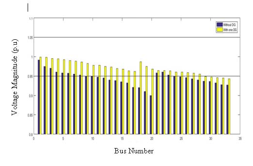
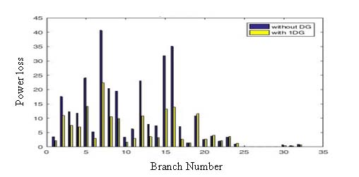
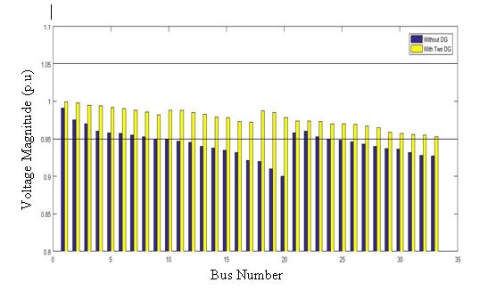
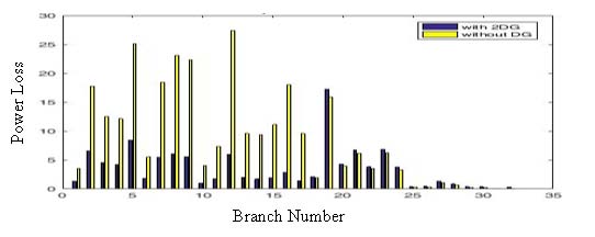
16. Results for Optimal Placement and Sizing of dg
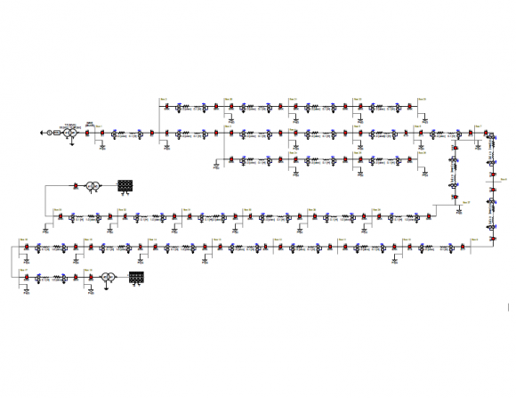
To verify and validate the effectiveness of the developed MPSO based optimal placement and sizing of DG. Load flow studies were conducted using Hybrid combination of Back ward -Forward sweep with Newton Raphson method to determine power losses in the test system. MPSO was used to determine the optimal location and size of the DG considering two cases to reduce power losses and to improve voltage profile. The results for DG placement are shown in Tables 3.
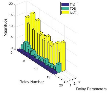
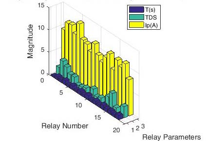
17. XI. Coordination Simulation Results
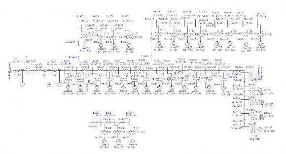
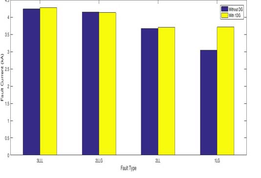
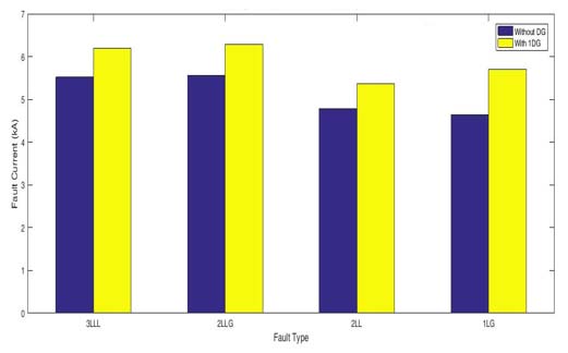
To investigate the impact of DG on protection coordination, the networks were modelled and simulated using ETAP software for three different distribution networks. The sequence of operation of the protective devices for three phase to ground fault is as shown in Table 5.
18. Ferro Resonance Simulation Result
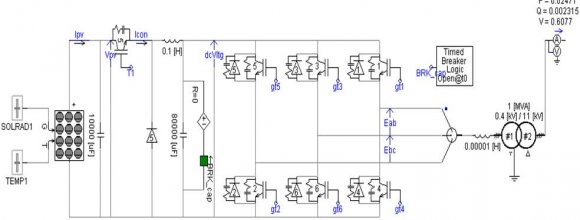
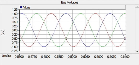
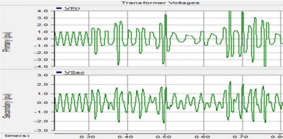
To verify the existence of Ferro resonance in the distribution network when there is circuit breaker or fuse failure, part of the network was simulated using PSCAD.
At the 33/11 kV injection substation with 7.5 MVA power transformer, switch was opened on phase B at the time of 0.1s and closed at 0.5s. The bus voltage and the transformer primary and secondary voltages were plotted in Figures 14 and 15.
19. Reliability Evaluation
To investigate the reliability of the system, the following reliability indices of the systems were evaluated using ETAP: System Average Interruption Duration Index. System Average Interruption Frequency Index, Expected Energy Not Supplied and ECOST.
20. Reconfiguration Results
Optimal number of switches and their locations is presented in Table 7. One solar power DG with optimal size as suggested by MPSO was connected to the model of the network at the optimal location. As a result of a fault introduced at a bus immediately after the bus with DG, fuse A3 opened after the third operation of the autorecloser at the beginning of the lateral. To reconfigure the network, SW A3 was manually closed. The model of the network used for the simulation, the number of buses isolated as a result of the fault and the corresponding number of customers and the number of buses restored and the corresponding number of customers are presented in Table 8.
21. XVI. Network Reconfiguration Results
for IEEE 33 -Bus Test System with Two DG
Two solar power DGs with optimal sizes as suggested by MPSO was connected to the model of the network at the optimal locations. As a result of a fault introduced at a bus immediately after the buses with DGs, fuse A2 opened after the third operation of the autorecloser at the beginning of the lateral. To reconfigure the network, SW A4 was manually closed. The model of the network used for the simulation, the number of buses isolated as a result of the fault and the corresponding number of customers and the number of buses restored and the corresponding number of customers are presented in Table Table 8
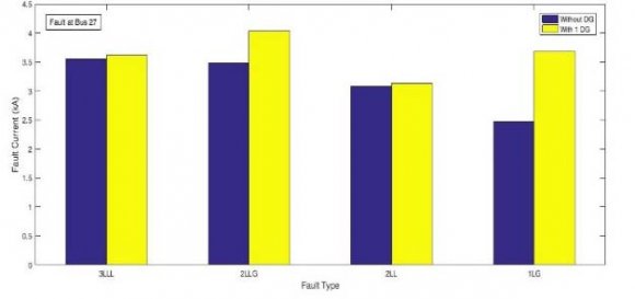
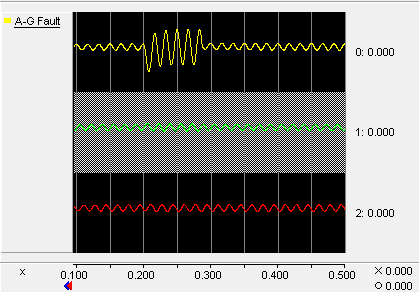
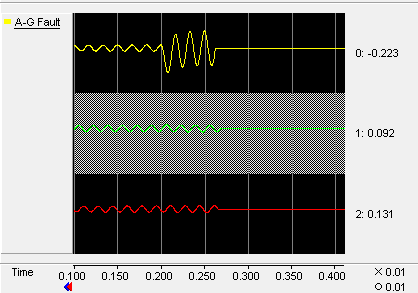
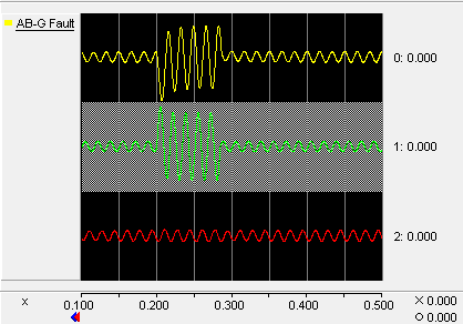
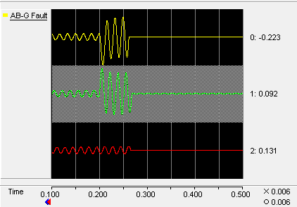
22. Results on Development of Adaptive Protection Scheme
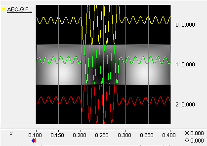
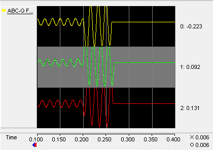
To validate the models created in PSCAD, the bus voltage at each of the buses were compared with the ones obtained using ETAP. And different simulation cases were performed to test the performance of the proposed adaptive protection schemes. Simulations include relay setting update for system configuration change, faulted section identification and interruption by the appropriate breaker. The simulations cases were performed to test all the three distribution systems as follows: The results for the fault current, breaker interruption and relay settings update are all plotted.
The network was modelled using PSCAD. Three cases were simulated for this network. The fault current seen by the relays, the interruption by breaker and the relay settings update were all plotted in Figures 17 to 22. Conclusions DG are often used as back-up power to enhance reliability or as a means of deferring investment in transmission and distribution networks, reducing line losses, deferring construction of large generation facilities, displacing expensive grid supplied power, providing alternative sources of supply in markets and providing environmental benefits. However, power distribution systems integrated with DGs are always subjected to changes in the system configuration. During fault clearance or maintenance requirements, certain DGs might get disconnected. The changes in the configuration may lead to significant changes in the fault current level, which cause mis -coordination and malfunctioning of the previously coordinated directional overcurrent relays. To maintain proper coordination, protection relays should change their settings automatically whenever a change in the power system configuration occurs. Therefore, in this work, communication based adaptive protection scheme that can update the relay settings in accordance with the configuration of the network is proposed for distribution network with distributed generation.
Herein, MPSO was developed to optimally sized and sited DG which provides minimum power loss and enhanced voltage profile. IEEE 33 bus test system was used to test the effectiveness of the technique by integrating one DG and two DGs. And finally deployed for two Nigerian distribution networks: University feeder in Maiduguri and Ran feeder in Bauchi. The optimal location, DG size and percentage power loss reduction obtained for the IEEE 33 bus test system when single DG was integrated is bus 22, 2.59 MW and 47.3 % respectively when differential evolution was used while bus 28, 1.89 MW and 48,85% respectively when MPSO was used. For the second case i.e. integration of two DGs, the optimal location, DG size and percentage power loss reduction are buses 20 and 25, 1.58 and 0.97 MW and 50.6% for differential evolution and buses 18 and 33, 1.41 and 0.51 MW and 71.51% for MPSO. It can be concluded from the analysis that MPSO is gives better results in terms of power quality.
In this research, effort has also been made to model the three networks in both ETAP and PSCAD environment and evaluate the impact of DG on the protection systems when DG is integrated in the systems. The type of DG integrated was solar photovoltaic and Hydro power systems. The result shows that there was change in the fault current level and there was unintentional islanding and false tripping as a result of the current contribution from the DG.
The final goal of this research work concerned with the development of adaptive protection scheme for distribution network with DG using PSCAD. The operation of the adaptive protection scheme was verified through several simulation cases. The experimentation was carried out by conducting ten scenario cases with four different fault types. The simulation studies yielded far-reaching results that have been exhaustively discussed.


| Characteristics (IEEE Standard C37, 2002 | |||
| and IEEE Standard 1366, 2012) | |||
| Characteristics | A | B | P |
| Moderately Inverse | 0.00515 | 0.114 | 0.02 |
| Very Inverse | 19.61 | 0.491 | 2.0 |
| Extremely Inverse | 28.2 | 0.1217 | 2.0 |
| ?? ?????? = ?? ð??"ð??"????ð??"ð??"?? ? | ?? ð??"ð??"????ð??"ð??"?? ? ?? ?????? ??????ð??"ð??" ?????? | × ??????ð??"ð??" |
| Where, | ||
| ?? ?? , |
| S/No | Parameter | Value |
| 1. | Maximum iteration | 50 |
| 2. | Particle size | N |
| 3. | ?? 1 , ?? 3 , is the cognitive acceleration coefficient | 2 |
| 4. | ?? 2 , ?? 4 is the social acceleration coefficient | 1.5 |
| 5. | ?? 1 , ?? 2 , ?? 3 , ?? 4 are n dimensional Colum vectors | 0.8 |
| 6 | W is the static inertia weight | 0.9 |
| 7 | ?? 1 , ?? 2 ,?? 3 , ?? 4 matrix for best particle | [1, 1, 0, 0] |
| 8. | ?? 1 , ?? 2 ,?? 3 , ?? 4 matrix for bad particles | [0, 0, 1, 1] |
| 9. | Maximum inertia weight | 1 |
| 10. | Minimum inertia weight | 0.6 |
| VII. |
| S/No | Parameter | Single DG | Two DG |
| 1 | Best Location | Bus 28 | Bus 18 and 33 |
| 2. | DG size (MW) | 1.87 | 1.41 and 0.51 |
| 3. | DG Type | Solar | Solar |
| 4. | Initial power loss (kW) | 221.43 | 221.43 |
| 5. | Final power loss (kW) | 101.1 | 80.21 |
| 6. | % Power loss Reduction | 48.85 | 61.51 |
| S/No | Parameter | Without DG | With 1 DG | With 2 DG |
| 1 | Bus violating limits | 18 | 5 | 0 |
| 2 | Sum of square of voltage error | 0.1369 | 0.02968 | 0 |
| 3 | Total number of customers affected | 1944 | 843 | 0 |
| Number of | DG | Fault | Actual tripping | Correct Tripping | ||
| DG | Bus | Bus | Primary | Backup | Primary | Back up |
| One DG | 28 | 29 | Fuse 3 | DG1 Relay Main Relay | Fuse 3 | Lateral Recloser3, Main Relay |
| Two DG | 18 & 33 | 19 | Fuse 4 | Lateral Recloser 1, Main Relay | Fuse 4 | Lateral Recloser1, Main Relay |
| Two DG | 18 & 33 | 34 | Fuse 3 | DG2 Relay, Main Relay | Fuse 3 | Lateral Recloser 3, Main Relay |
| XII. |
| S/No | Distribution Network | Number of Switches | Switch Locations |
| 1. | IEEE 33 Bus Test System | 11 | SW2,SW3,SW5,SW6, SW7, SW8, SW10, SW11, SW12, SW14, SW16, |
| XV. Network Reconfiguration Results | |||
| for IEEE 33 -Bus Test System with | |||
| Single DG | |||
| XVII. | ||||||
| Parameter | Number of | |||||
| DG | ||||||
| Base Case With | One | With | Two | |||
| DG | DG | |||||
| SAIFI | 1.8977 | 0.5231 | 0.4470 | |||
| SAIDI | 8.2084 | 3.4424 | 3.0293 | |||
| CAIDI | 4.326 | 6.581 | 6.776 | |||
| EENS | 29.336 | 16.147 | 11.211 | |||
| ECOST | 112,970.40 73,976.11 | 40,872.68 | ||||
| ASAI | 0.9991 | 0.9996 | 0.9997 | |||
| ASUI | 0.00094 | 0.00039 | 0.00035 | |||
| AENS | 0.1424 | 0.0784 | 0.0544 | |||
| Parameters | Number of DG Single DG Single DG Two DG | Two DG | ||||
| Fault Bus | 29 | 29 | 16 | 16 | ||
| Sectionalizing Switches opened | Recloser A3 | Recloser A3and Fuse A3 | Recloser A3 | Recloser A2 and Fuse A2 | ||
| Tie Switches Closed | - | SW A3 | - | SW A4 | ||
| Number of Buses isolated | 8 | 4 | 9 | 4 | ||
| Number of Buses restored | 0 | 4 | 0 | 5 | ||
| Number of Customers isolated | 46 | 24 | 1042 | 621 | ||
| Number of customers restored | 0 | 22 | 0 | 421 | ||