ince the beginning of the space era, the space environment around Earth became a junk yard full of debris related with space missions. Debris were generated due to explosions (deliberated or not), launch vehicle upper stages, inoperative satellites and even tools and small objects. The millimetre and submillimetre source of debris are propellant residuals, fragmentation processes and ink fillets detached from spacecrafts surface. In 2004 about 40% of debris were generated by explosions and collision involving launch vehicle upper stage or spacecraft in orbit (Bendisch et al., 2004).

The satellite Sputnik 1 launched in 1957 became the first space debris produced by men. 4 years later this launch, the space around the earth had become populated with 300 debris resulted by the explosion of the American Transist-4-A rocket, an explosion which happened 2 hours after reaching orbit. Today, after over 4,900 launches, the space activities produced about 240 further explosions which form the main source of production of space debris (ESA, 2013). With the space race, even with mitigation measures and the natural atmospheric drag in the objects in LEO the distribution of objects in the operating regions increased.

The vehicle propulsion system is responsible for 45.7% of the fragmentation that occur mainly due to catastrophic damage during orbit insertion or others manoeuvres, also there is factors related with failure of the active control system. The growth rate of fragmentation increased since 1970 achieving 5 fragmentation per year (Johnson et al., 2004). Collisions with debris larger than 10 cm are still considered catastrophic and consequently come up a cascade process of other collisions. This type of collision cascade process produces a critical density in long time, and without reduction perspectives, unless the amount of large objects is reduced.

In view of the great need of space missions some control techniques must be adopted to avoid the growth of debris in the operating regions (Kessler and CourPalais, 1978;Kessler, 1991). Simulations indicate that in a few decades debris from collision fragments will dominate the Earth space in attitudes between 800-1400 km at least (ESA, 2013). It is clear that the damage to space missions are large, even for smaller debris, since they may disable or burst operational vehicles and can make infeasible a space mission.

The distribution of space debris in LEO, MEO and GEO altitudes causes concerns about the safety of space activities operations in these regions. The size and altitude of debris are crucial in observing and tracking by radars. Depending on the accuracy and ability of the radar, smaller debris can be catalogued in higher altitudes. Optical instruments and radar are able to track and catalogue objects of sizes between 5 and 10 cm in LEO and sizes between 0.3 and 1 m in GEO (ESA, 2013). This indicates that the latter region can be populated by smaller and potentially destructive objects not catalogued. In fact, more than 99% of the mass and area of the population in orbit actually are debris which potentially capable of producing catastrophic rupture (Kessler, 1991).

In MEO region orbits the navigation constellations (GPS, GLONASS, etc.) and about 16,000 debris with diameters larger than 1 cm are predicted to cross orbits in this region. Most of them have non-zero eccentricities, causing them to reach altitudes of GPS in its apogee. The energy produced in a collision is about 104 J which could cause severe damage to the spacecraft (Klinkrad, 2006;Rossi, 2005;Rossi and Valsecchi, 2006;Smirnov, 2001). The orbital perturbations in GEO region, different from the atmospheric drag in LEO, does not reduce the amount of debris (Milani et al., 1987). Since the launch of Syncom-3 in 1964, more than 800 satellites and rocket stages were placed in this region. The growth rate GEO debris without removal, increases 30 debris per year (Valk et al., 2009).

It is clear that security measures must be taken and evasive manoeuvres must be planned to prevent accidents among spatial objects. The collisions between operational vehicles with space debris became a reality, although in the point of statistical view they are rare. In most cases, on average ten risk alarms are generated per year, and fewer avoidance maneuver are implemented by year (ESA, 2009). But these estimates depend on a combination of many factors and specialized computer codes.

Beyond that there is a lot of uncertainties such as debris related with non-commercial missions, that is, upper stages and debris linked to certain classes of American secret missions and, more recently, a couple of Japanese reconnaissance spacecraft, which are not included in the catalogue version available (maintained by the Space Control Center, operated by the Air Force Space American Command) to commercial and foreign entities (Godwin, 2003). This account for approximately 4% of the catalogued objects. And there are other uncertainties that affect the missions in LEO, for example, modelling the uncontrolled satellites trajectory by re-entry, distortions in the observation of debris that occur in long time observation, the difficulty in predicting solar and geomagnetic activities which depends on the atmospheric density (Rossi et al., 1998;Anselmo and Trumpy, 1986).

This paper studies evasive manoeuvres in operating regions to establish technological parameters that are efficient to implement. This is a first model without dissipative forces in all regions.

Our study does not include dissipative forces, as it aims to establish optimal conditions for the evasive maneuvers of a vehicle in front of the possibility of collision with space debris. Moreover, the study is restricted to collisional bodies whose relative distance between them is smaller than the spacecraft to the Earth.

Our approach is based on the study of the relative movement between a vehicle and a space debris. The reference system in Figure 1 is fixed on the vehicle. We measure the positions and relative speeds w.r.t. this system, such that all technical control evasive maneuver is performed from it. The dynamics between these objects not consider active dissipative forces, only the Earth's gravitational force on the vehicle and the debris and the propulsive force of the vehicle.

We consider that the relative distance between objects is very small com-pared to the distance from the vehicle to the center of the Earth, that is, ( ?? ?? << 1). In this condition, the resultant force of gravitational term can be expanded and analytic solution may be found with significant accuracy (Clohessy-Witshire, 1960). The thrust adopted in our model is proportional to the rate of exhaustion of the propellant vehicle system and, through it, the movement can be controlled. The equations for the Cartesian components of the relative acceleration are:

(1)

Figure 1: Reference frame for a vehicle around Earth and for a space debris. The frame with capital letters is positioned in the Earth center.

(

These Equations model the relative dynamics between operating vehicle and space debris. For each orbital region (LEO, MEO, GEO) the vehicle orbits side of these Equations are the components of the nongravitational acceleration, in which case the components of the acceleration of propulsion. For this dynamics, we adopt exponential change in mass of the vehicle in time, such that,

With m o as the initial propellent mass and ? is the power factor of the engine. The total mass of the satellite is dependent of the mass of the propellent:

(

With M o is the net mass of the satellite disregarding the propellent.

We write the mass factor as ( 6)

And then we have (7) The technological parameters identified for this dynamic are:

1. Components of the gas exhaust velocity 2. The power factor of the engine ? > 0 and; 3. And the mass factor ( ), that is, the mass ratio between the spacecraft mass (M o ) and the initial propellant mass (m o );

The components of the propulsion force are,

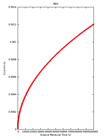
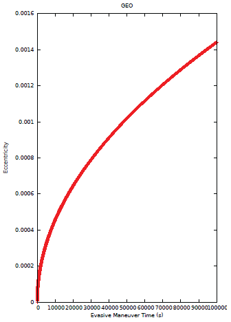
These Equations show that the evasive maneuver can be controlled by the power factor, maintaining the circular or quasi-circular orbit. We found that for circular orbits in LEO, the value of optimal power factor is 10-6 (Jesus et al, 2012). This factor should be reduced to that circular orbits nearly circular or are kept in MEO and GEO, as we shall see. In the Appendix, we show the evolution of the eccentricities of the orbits of these operating regions for our model.

The necessary condition for the collision between two space objects (operational vehicle and space debris) is its final position relative to cancel an instant t c , ie, (11) This condition must be satisfied concerning the dynamics through a set of initial conditions that includes the components of velocity and position on the objects. The initial relative position is calculated by scanning the spherical angles (in-plain, , and out-plain, , distributed in the region of space where the collisional objects. The relative initial velocity can be found as a function of time through the homogeneous solution of Equations ( 1) to (3) to F x = F y = F z = 0. We call this set, including the tc, set of initial conditions collision course (CICC). The CICC elements constitute the collision possibilities in the dynamics on these objects, subject only to gravitational force. It does not determine the collision probability, because the equations of speeds are deterministic and not probabilistic. It admits the collision possibilities in the relative dynamic. Thus, the set (CICC) is obtained by the distribution possibilities in the collision time, mapped by a function of the type, (12) Each pair (

) provides a possibility of collision between objects. We found the inhomogeneous solution of the Equations (1) (3), whose Cartesian coordinates are:

These are the Cartesian components of the final relative position of the objects subject to gravitational and propulsion forces. This vector determines the separation of the objects at each instant. In tc, determines whether a collision has occurred. All coefficients of these equations depend on the initial conditions and the technical parameters that can generally be written as Therefore, the condition (5) can be controlled from the set of these coefficients through technological parameters suitable for the implementation of evasive maneuvers. These maneuvers are possible every time the final separation between the objects is comparable to the dimensions of them. In this paper, we consider the collisional objects as known-radius spheres.

An operating vehicle in collision with space debris must implement an evasive maneuver to avoid it. The radar installed at the base on Earth or on the vehicle will provide information about the initial relatives position and velocity, and the collision time, tc. The satellite onboard computer will perform calculations on the possibility of collision and also indicate the coordinates that allow the escape of the collision. In this work, we simulate these conditions, setting the time of collision

and getting the initial conditions in favorable velocities and positions to the collision. Hence, we simulate the dynamics described in Equations ( 7) to (9) to implement the evasive maneuver.

Our numerical simulations of evasive maneuvers followed the following general steps: 1. Chose the orbital region (LEO, MEO, GEO) where collisional objects are and calculate the angular velocity that characterizes; 2. Use the solutions of the homogeneous equations of relative dynamics to calculate the initial relative velocity that allow collisions; 3. Set the collision time and the relative initial distance, r o , between collisional objects and found angles ( ), consistent with collisions between objects; 4. Calculate the components of the initial relative position from their values; 5. Select a pair of initial conditions of the CICC set, Equation ( 6), and t c ; 6. Chose specific technological parameters for the orbital region; 7. Implement the evasive maneuver the spacecraft, operating the propulsion system, numerically simulating the Equations ( 7) -( 9); 8. Obtain the final value of the relative position between objects, testing the collision condition (5).

With these steps we intend to model approximately the realistic conditions of an evasive maneuver on the possibility of a collision. To scan the entire sphere of radius with pairs of angles ( ),is performed to select those that enable collision. Technological parameters are extracted from the catalog-curves produced in this paper, consistent with the limits for circular or nearcircular orbits. They characterize the propulsion system of the vehicle and are used to control their escape from the collision.

The numerical simulation of evasive maneuvers should take into account information on the initial conditions, the time of collision and the characteristics of the propulsion system, represented by the technological parameters. The collision time should be small compared to the orbital period and sufficient for the evasive maneuver is implemented. Each element of the set CICC is a possibility of collision. The choice of this element is not arbitrary, why should characterize a real collision in orbital regions. For the numerical simulations, we chose the initial relative velocities equal to (7,76 km/s, 4,25 km/s, 1,01 km/s) in LEO, MEO and GEO, respectively, non-planar maneuvers which they are typical in these regions. We investigated the possibility of collision in a higher range of these velocities, that is, [1,0 -20,0 km/s].

The evasive maneuver is characterized by technological parameters (

), with which you can control these maneuvers front of an imminent collision. Equation ( 6) is valid for any time. The typical technological information space missions can restrict the solutions to a finite set. The observations of radar confirm average values of initial relative velocities specific to each operating region and also the minimum time required to perform the operations for evasive maneuvers. Thus, the simulations will be carried out in finite time and collision possibilities will also be finite, although in large numbers.

In this section we show the results of numerical simulations of the relative dynamics between two collisional objects (vehicle and space debris).

The results show: 1) the distribution of collisions in relative initial velocities ranges; 2) a parametric analysis of evasive maneuvers, characterizing the efficiency of the propulsion system that implements them. In the distribution of collisions we call collision possibilities. In implementing the evasive maneuver only use one of them. Figure 1 shows a reference system centered on the space vehicle. In its origin it focuses a sphere of radius equal to the relative distance between the vehicle and the space debris. Thus, our simulations vary these distances between 3 and 500 km, with initial relative velocities between 0 and 20 km/s. Knowing the collision possibilities in their collision time, we conducted a systematic study of technological parameters that are appropriate for the implementation of various evasive maneuvers. From there, curvescatalogue are generated, considering the variation of these parameters over time and size of collisional debris. For each operating region (LEO, MEO and GEO) choose an element of CICC to implement the evasive maneuvers in the region. In this work, we simulated various evasive maneuvers, taking into account debris and space vehicles of different dimensions. The evasive maneuvers will be confirmed based on the final values of the relative positions, comparing them to the sizes of the space objects.

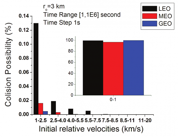
The possibilities of collision between the space objects (vehicle and satellite) are high, considering a time interval of 10 6 s. Figure 2 below shows the distribution of collisions depending on the initial relative velocities interval between objects for the operating regions. For discussion purposes, we divide the range of relative initial velocities, as follows: 1) low velocitiesbetween 0.0 and 4.0 km/s; 2) medium velocitiesbetween 4.0 and 7.5 km/s; 3) high velocities -between 7.5 and 10.0 km/s, and; 4) high velocities -between 11.0 and 20.0 km/s.

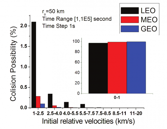
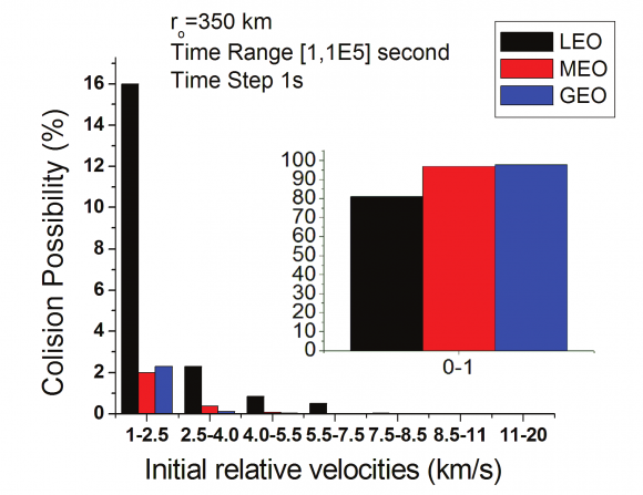
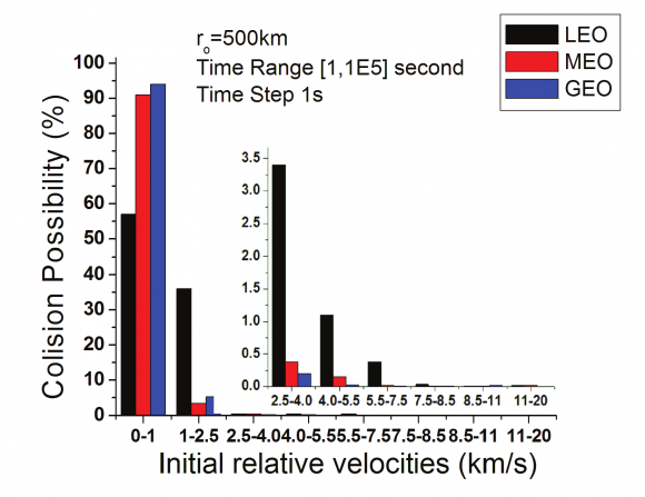
In Figure 2, we note that for any operating region there is little chance of collision for high and very high initial velocities, if the objects move away initially 3 km. This result is consistent with the expected, since the velocities decrease with increasing altitude. Moreover, in The same is true for MEO regarding GEO. Obviously, the effect of the Earth gravitational field, favors the approach of objects in LEO by increasing the collision possibilities. For the range of initial velocities nulls or nearly nulls, the collision possibilities are virtually the same for any operating region. Figures 3, 4 and 5 show the results of simulations for other initial relative positions between the space objects to collision time equal to 10 5 s. This collision time is compatible with orbital periods in MEO and GEO. For LEO it would be 10 3 s. These results generalize those for r 0 = 3 km. That is, the collision possibilities for high and very high velocities are small to any initial relative position. Proportionally, these collisions occur, possibly in LEO more than MEO, and MEO more than GEO. For medium velocities, there is greater possibility of collision if the objects are initially farther away and at higher altitudes. Thus, we say that a greater risk scenario is established for imminent collision in any relative initial velocity, especially in LEO, MEO and GEO followed. Moreover, our model does not include dissipative forces occurring in these regions. These forces interfere with the distribution of physical initial conditions that enable collisions, sometimes favoring them, sometimes reducing them. Our simulations did not include these forces, and thus our results are an ideal initial test, establishing physical and technological conditions for complete dynamics with dissipative forces.

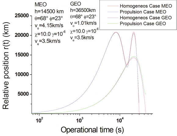
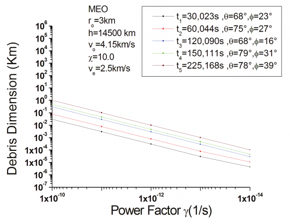
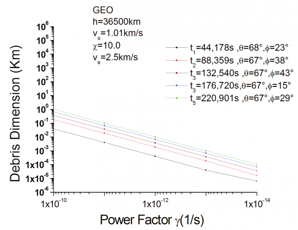
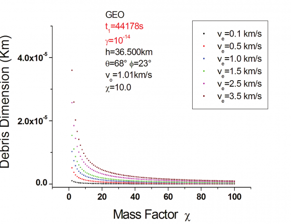
Knowing the dimensions of the collisional objects, our model determines if the evasive maneuver is sufficient to avoid collision between them. The technological parameters are used to evaluate the feasibility of evasive maneuvers for the set of initial conditions favorable to the collision, the collision time interval. For this study the technological parameters, simulated evasive maneuvers between objects initially separate to 3km, with angles ? = 68 and ? = 23 degrees in MEO and GEO regions. The equivalent study for LEO was held earlier paper (Jesus et al., 2011). The red and pink curves, Figure 6, represent the course of a collision (homogeneous solution of Equations 1, 2 and 3) between the objects in the initial conditions for the MEO and GEO regions, respectively. Curves in blue and green represent their evasive maneuvers, whose initial relative velocities are typical of these regions (4.15 km/s -MEO and 1.01 km/s -GEO). These curves characterize the dynamics with propulsion to escape collision with space debris. They inform the final relative position between collisional objects at each time, obtained by the performance of operational vehicle propulsion thrusters. We note that collisional objects initially separated to 3km escape of the collision at different times and in different operating regions. Moreover, their final relative distances are different, which can characterize different sizes of debris. We note that the curves with propulsion characterize success of evasive maneuvers, as the final relative positions are not zero. This success is in large collision time, such that the continuous propulsion can overcome the gravitational effects on the objects, setting their final relative position and avoiding the collision between them. In all cases with propulsion, the collision is easily avoided in hundreds of kilometers of separation between the objects to these maneuvers under these initial conditions. The maneuver MEO escapes closer to the collision in relation to maneuver in GEO. This fact is associated with the typical initial relative velocities and also the period orbits in these regions. The qualitative behavior shown is general, although the results are specific to these regions with the given initial conditions. Thus, we say that given the initial conditions favorable to the collision, the objects develop a relative dynamics to propulsion, such that as time passes, they leave the collision course, swaying their positions around it to fully escape, featuring the evasive maneuver. These initial conditions are overcome by the performance of the propulsion system. Therefore, the technological parameters of it were efficient in the implementation of the evasive maneuver. Technological parameters are effectively crucial in the implementation of evasive maneuvers. They are related to the propulsion system of the space-craft and the correct choice of these parameters will allow efficient evasive maneuvers. The parameter characterizes the frequency with which the fuel is consumed in time, such that the higher it is, more fuel will be spent on the evasive maneuver. Figures 7 and 8, below, are catalogcurves which show the behavior of this factor as a function of collision time and the size of the debris in MEO and GEO, respectively. The results show that small power factors favor evasive maneuvers on a collision course with small debris. Conversely, evasive maneuvers to larger debris will require major power factors. This phenomenon occurs in both operating regions, MEO and GEO. It should be noted, however, that the increase of this factor in continuously burning regime can remove the operating object of their nominal circular orbit. In this model we chose power factor operation MEO and GEO equal to 10 -10 (see Appendix), which ensures the permanency of the operating object in a circular or nearly circular orbits. Moreover, very small power factors prevent the implementation of the evasive maneuver, since the propulsion force is virtually zero. But observing such limits, evasive maneuvers can be performed efficiently to escape collisions with debris of various sizes, depending on the time of collision and the propulsion system characterized by the parameter. We say that the high power factor would favor evasive maneuvers with less risks of collision with cloud debris of any sizes. Another technological parameter that we consider is the mass factor. This quantity measures how much the vehicle mass is greater than the initial mass of the fuel it carries. Figure 9 shows the relationship between this factor to the size of the debris which evasive maneuvers escape into GEO, and the exhaust velocity. The power factor used here is equal to 10 ?14 .

In this Figure we observe that evasive maneuvers with small mass factors are more efficient to escape debris increasing relatively. Higher exhaust velocities are favorable to these maneuvers. To escape of smaller debris, lower exhaust velocities are preferable. However, large mass factors are favorable to the evasive maneuvers against collisions with smaller debris and this is independent, practically, the increasing values or not the exhaust velocities.

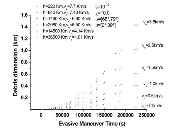
The results obtained here for MEO and GEO are equivalent to those found by Jesus et al. (2012) to LEO. Figure 10 below shows the risk curve in LEO, MEO and GEO, under the action of gravity forces and propulsion. They are ideal curves because it does not consider the dissipative forces occurring in these regions. In this curve the dimensions of the debris are distributed as a function of collision time, of altitude and of the vehicle exhaust velocities. We note that the qualitative behavior of the curves remains for any altitude of collisional objects and the quantitative results are a function of exhaust velocity.

We note that with higher exhaust velocities will be possible to escape from collisions with large debris. This means that more powerful propulsion systems are less efficient and less economic for evasive maneuvers in small sizes debris environments. In addition, we observed that the risk of colliding with large sized debris increases with low velocities. This risk is reduced by increasing the exhaust velocities. Therefore, it is preferable and more economical to use small exhaust velocity, since the power of the propulsion system must be preserved for escape maneuvers against collisions with very large sizes of debris. Hence, the need for a propulsion system capable of con-trolling the magnitude of velocity in non-uniform size distribution of debris environment.

The risk curve, shown in Figure 11, provides information that can be used in decision-making on a space mission to avoid collisions with space debris. To use this curve should be chosen initially, one octant. In this curve, we choose the angles in-plane and out-plane within the range 68 to 79 degrees and 6 and 39 degrees, respectively. Our results showed that the qualitative behavior displayed in this curve is general for all octants, where are located the collisional objects. There is a relationship between the dimensions of collisional debris with the collision time for every operating region. The exhaust velocity is the coefficient between them. It is essential in the implementation of evasive maneuvers, since it is related to engine power. The use of the risk curve in space missions must follow an algorithm of operations that allow to perform an evasive maneuver. If the propulsion system for variable velocity, so the operating system of the vehicle will have the freedom to make decisions to escape from any debris, based on the information on the collision time. The radar informs the coordinates of the debris and the collision time. The vehicle would be in a specific altitude, for which there is a specific curve as a function of Global Journal of Researches in Engineering ( ) Volume Xx X Issue I V ersion I D exhaust velocity. Thus, based on the collision time and the vehicle altitude the operating system know whether or not escape the debris, depending on its size. The onboard computer will calculate the escape trajectory and the curve will inform if one can escape the specific size debris and this will depend on the velocity that the propellant system is able to implement. If the thruster system is not able to vary the exhaust speed, there will only be a range of sizes of debris it can escape. This range is as large as is the variation of the exhaust velocity values.

V.

Our results showed that the relative dynamics between a vehicle and space debris is rich in collision possibilities in LEO, MEO and GEO. Thus, we say that a greater risk scenario is established for imminent collision in any relative initial velocity, especially in LEO, MEO and GEO followed. Our simulations did not include dissipative forces, and thus are an ideal initial test. The continuous propulsion can be used to avoid collisions with space debris, pro-vided that suitable technological parameters. These parameters can control the evasive maneuvers depending on the size of the debris and collision time. If the vehicle has short time to escape, the evasive maneuver occurs if in imminent collisions with small debris. In this case, small exhaust velocities are preferable. We found a risk curve for orbital maneuvers. This curve informs that a system propulsion with variable exhaust velocities is preferred for the evasive maneuvers. These maneuvers would be more economical and efficient to avoid the collisions with any debris.