1. INTRODUCTION
here has been remarkable research achievement in developing and applying computerized tomography (CT)technology for medical and industrial applications, particularly in the industrial area, such as aerospace, aviation, military, machinery and automobile. Industrial CT is not only effective to detect the inner construction and flaws of an object, but also necessary to nondestructively measure the size of workpiece [1,2]. However, the two dimensional slice images acquired by the 3rd generation ICT device can't be edited in the existing computer aided design (CAD) system. And most industrial CT images are the workpieces' dislocation images, which have many geometrical elements, such as lines, circular arcs and circles. Several conventional vectorizaion methods, applied in engineering drawings and maps, come with disadvantages, including noise sensitivity, computational complexity and low accuracy. These shortcomings make it difficult to accurately measure the size of workpieces' inner construction. In order to overcome these problems, in this paper we investigate methods of industrial CT images precise vectorization.
Since the research of image vectorization started in the early 1970s, numerous approaches have been developed [3,4]. Broadly, these algorithms can be divided into several groups: thinning algorithm, contour tracking, Hough Transform (HT), dynamic window method and global recognition algorithm. The main advantage of thinning algorithm is that it holds a better reservation of image topology information, and its processing data points are decreased. Nevertheless, it is sensitive to noise. As a solution of this problem, the contour tracking method is provided. Its processing rate is high, and the impact of the air bubble and burr defects on the vectorization effect is reduced. However, the recognition accuracy is low since the vector image is discontinuous. In terms of accuracy and robustness, the HT and its variants have been successfully used in image vectorization. These methods are robust against outlier and occlusion, but computationally expensive. Dynamic window vectorization algorithm was proposed as a relatively novel method. A major advantage of this method presents at its high recognition accuracy to crossing point. Unfortunately, the window is changing continually, so the robustness is not enough. With the vectorization technology improving, some researchers have presented global recognition method. In process of vectorization, the line width can be obtained. Meanwhile, the corresponding tracking mode is adopted for reducing the impact of line fracture and missing data. But the accuracy of crossing point should be further improved.
In view of the disadvantages of the current image vectorization methods, the key contribution of this paper is to investigate a vectorization system for industrial CT image. In this system, the sub-pixel edge of an industrial CT image is extracted based on facet model. Its execution time is reduced significantly by removing invalid data points. Then, the circles, lines and circular arcs are recognized respectively with the corresponding recognition algorithms. These algorithms improve recognition accuracy. Also, in the process of recognition, the obtained elements parameters are dynamically saved in the corresponding linked lists. Hence, the required computation storage space is much cheaper than the previous methods.
2. II.
3. SYSTEM OVERVIEW
In the process of industrial CT image vectorization, it is critical to detect edges in the image which is an important stage as the quantity and quality of edge data will affect greatly the vectorization performance of the system. The sub-pixel edge contour is extracted by the edge detection algorithm based on facet model, after the pre-processing as Gaussian filter, binarization. For this contour, the recognition algorithms of graphic elements are implemented. Firstly, determine whether the contour is a circle by calculating the center's probability. If it is a circle, the improved fast algorithm of circle detection based on probability of existence map is utilized to recognize it. The obtained circle parameters by the least squares function (LSF) are saved in the circle chained list. Reversely, if it is not a circle, the contour curve is fitted into many short line segments by adopting the improved set intersection algorithm of fitting a straight line. Then, merge the short line segments into the long line segments. Finally, the perpendicular bisector tracing algorithm is adopted to find the long line segments which can be fitted into circular arcs. And the merged circular arcs' parameters are derived from the least squares function. These parameters are saved in the circular arc linked list. Another long line segments' parameters are saved in the line linked list. After recognizing these elements, their parameters are outputted for vector graph. The system architecture is summarized in Fig. (1).
4. EDGE DETECTING ALGORITHM BASED ON FACET MODEL
The exact location of edge is obtained by using the edge detection algorithm based on facet model. Through calculating the second-ordered directional derivative, edge point is defined as the zero-crossing point of facet model along the gray gradient direction [5]. Third-ordered facet model of the pixel (x, y) in 5×5 regions can be expressed as follows:
(1)
Where (r, c) is the coordinate of any point in this pixel's neighborhood; k1~k10 are the coefficients which are obtained by the least square method [6]. So (2) Define r = ! sin" ,c = ! cos" (? is the distance between edge point and the center of pixel), the firstordered, secondordered and third-ordered partial derivatives of the model can be expressed as follows:
(3)
The edge point is the location of local extremum of the first-ordered derivative in local fitting surface; meanwhile it is the zero-crossing point of the secondordered derivative as well. (r, c) is the edge point, if we can obtain ?0 (?0 is within the 5×5 sub-region whose center is (r, c)) which satisfies (4), and the third-ordered partial derivative negative, as in ( 5).
(4) (5) Adopting this algorithm, the subtle image detail is located. The edge detection accuracy is high enough, and the image noise is restrained to some extent.
IV.
5. RECOGNITIION OF GRAPHIC ELEMENTS a) Recognition of Circle i. Existence Probability of Circle
Circles in the X-Y plane can be completely represented by the following quadratic equation with three parameters (u,v, r) as other 2nd order curves can be.
(
)6In order to obtain the size and position of circles in industrial CT image, the method based on probability of existence map is applied [7]. Pe is the existence probability of the circle whose center is (u, v) and radius is r. It is given by: (7)
Where A(r ) is the amount of edge points, whose distance from the center equals r; 2?r is the amount of discrete pixels of the circle with radius r.
Every pixel (x, y ) in the image is regarded as the center, the existence probability Pe is calculated and saved in the two dimensional array {P (x, y )}. The probability of existence map is produced, and the radius r is saved in the two dimensional array {R(x, y )}. Each peak in probability of existence map represents that a circle may exist in this image, taking the peak coordinates as the center and r as the radius. Pe is the probability of such existence. August ii. Improved Algorithm of Existence Probability
f (r, c) = k 1 + k 2 r + k 3 c + k 4 r 2 + k 5 rc + k 6 c 2 + k 7 r 3 +k 8 r 2 c + k 9 rc 2 + k 10 c 3 r, c !["2, "1,0,1, 2] . sin! = k 2 k 2 2 + k 3 2 ,cos! = k 3 k 2 2 + k 3 2 f '(!) = m 1 + 2m 2 ! + 3m 3 ! 2 f ''(!) = 2m 2 + 6m 3 ! f '''(!) = 6m 3 " # $ $ % $ $ f ''(!) = 2m 2 + 6m 3 ! = 0 " m 2 3m 3 = ! 0 f '''(!) < 0 " m 3 < 0 (x ! u) 2 + ( y ! v) 2 = r 2 Pe = A(r) 2!The above algorithm regards each pixel in the image as the center of a circle, but most pixels in the image are not the center of the circle actually. As a result, the computation is complicated and the required computational storage is expensive. The center of the circle should lie in a mini-realm in the target region, thus, we improve the above algorithm by decreasing the select range of circle center to the square C [8]. If a closed curve has been recognized as a circle, the maximum distance of two points on the circle is defined as diameter, and the middle point of the diameter is the circle center. As illustrated in Fig. (4), for every closed contour, we first have to find the nethermost point A, then, calculate all distances from A to the other points. The point B that has the maximum distance D is the endpoint of the diameter. The midpoint O of the diameter is approximately regarded as the centroid of the closed contour. Therefore, a square C is obtained, whose center and sides are the centroid O and D × w (D = 100, w = 0.1), respectively. The square C is the area within which the potential circle center will be sought. In this way, the improved method constrains the search for potential circle center only in the specified small range and thereby reduces the computational cost. Besides, we improved the storage mode for saving memory space as well. Circle parameters, such as the coordinates of the circle center, radius and existence probability, are stored by a series of two dimensional arrays in the previous algorithm, which has to allocate memory beforehand. Thus, different types of images require different memory size. If the allocated memory is oversize, the memory space will be wasted; on the contrary, if undersized, memory space will cause data overflow. In this paper, we store the above parameters using the chained-list, referred to as the mode of allocating memory is dynamic, not beforehand. There is no need for this rule to redefine the memory size, even though the image size is different. As described in the following, the constructed list structure is effective in that it influences not only memory allocation, but also the recognition efficiency of a circle. After recognizing the circles in industrial CT image, the remaining contours are fitted into short line segments by an improved method of fitting a straight line. Based on the set intersection algorithm of fitting a straight line [9], the method makes use of least square technique [10] to get line segment parameters. Generally, the procedure of the method is as follows:
As shown in Fig. (5a). For a contour, the starting point is P 0 , the current point is P . At the beginning of fitting, P c =P 0. First, determine whether the next field of Pc is empty. If the next field is empty, end tracking the current line, get the line segment P 0 P c . If the next field isn't empty, judge whether the following point P n belongs to the current line. If P n is in the current line, then P n ?P c , and continue determining the following one. Or else, terminate tracking the current line, and get the line segment P 0 P c . Next, let P n be the new starting point, and continue recognizing other line segments of the contour. After finishing a contour recognition, the above process is repeated for another contour of industrial CT image. Due to low image quality and improper image preprocessing,the straight line may be mistaken as a series of short line segments, which we should merge into the long segments. The merging condition of two adjacent short line segments: the difference of slopes between two line segments must fall within the prescribed limits; and the distance between the endpoint of line segment and the merged long segment should be less than the specified value. As illustrated in Fig. (5b), if the angular difference between the adjacent line segments AB and CD is less than the prescribed value (using the angle value to represent the slope of line segment; here we choose 10°); and the distance from the point B to the line segment AC is less than the specified value (here 3 is appropriate), we will merge the short line segments AB and BC into the long segment AC. Then,determine whether the distance between the point C and the line segment AD is less than 3, and determine whether the angle difference between the line segment CD and the line segment AC is less than 10°. If the above two conditions are both met, get the long line segment AD. Or else, insert the merged line segment AC into the merged line link list, then, let CD be the new starting line segment, and continue merging the subsequent line segments.
6. c) Recognition of Circular Arc
The obtained short line segments by implementing the above strategy are merged into the long line segments. These long line segments are fitted into circular arcs by means of the perpendicular bisector tracing algorithm [11]. The basic idea of the algorithm is that the perpendicular bisector of any chord on a circle passes through the circle center, and every endpoint of the chord is at an equal distance from the circle center.
As illustrated in Fig. (6a), any obtained line segment may be an approximation of an arc. We first consider the obtained line segment L as seed arc, its perpendicular bisector P is constructed. For every line segments L (i =1, 2?N ), we then construct its perpendicular bisector P , and calculate the intersection C of P and P . Due to errors, the intersection C is not unique. However, all C are located along the line P . We define the point C is the nearest point from L , and the point C is the farthest point from L . Therefore, a rectangle C is obtained, whose length is the distance between C and C
, and whose width is equal to the length of L and is bisected by P . The rectangle C is the area within which the potential arc center is sought.
Fig. 6 (a) : Sketch map of circular arc fitting.
Having determined the potential center area, we check every pixel within it as a center candidate c (x, y ), the distances R i (x, y ) between c (x, y ) and endpoints of line segments are gained. Then, we calculate the average radius R (x, y ) and the mean square error ASD (x, y ), using ( 8) and ( 9), respectively.
(8)
The point whose ASD(x, y ) is minimal is taken as the circle center of circular arc, and the corresponding R (x, y ) is the radius of circular arc. The long circular arc may be recognized as some short circular arcs by using the perpendicular bisector tracing algorithm, so we merge these short circular arcs into the long circular arc. As shown in Fig. (6b), the merging condition of two adjacent short circular arcs: the coordinate difference between the circle centers O and O must fall within the prescribed limits (5 is fine); the radius difference between the radius R and the radius R should be less than the specified value (also 5 is enough); and the angular difference between the ending angle? of the first circular arc and the starting angle ? of the second circular arc should be less than the threshold value (the threshold value is 3°). If there are two circular arcs meeting the above-mentioned three conditions, they can be merged into a new longer circular arc. The new circle center coordinates of this longer arc can be defined by the average value of the circle center coordinates of the two shorter arcs, and the
i i i i i iradius of this new longer arc can be replaced by the average value of the radius of the two shorter ones. Also, the starting angle and ending angle of this new arc are substituted with the starting angle ? of the first arc and the ending angle ? of the second arc, respectively.
7. EXPERIMENTAL RESULTS AND EVALUATION a) Recognition of Circle
In this section, the performance of the proposed algorithms has been tested with the real industrial CT images. The algorithms are implemented in C++ with MS Visual C++ 6.0 complier on a desktop PC with AMD 64 processor 1.81GHZ and 512MB RAM. The vectorization system for industrial CT image is designed, which provides the platform for our experiments. Fig. (7a) is an original industrial CT image of a socket set by the ICT system of CD-650BX in Chongqing University ICT Research Center. The technical indexes of the ICT system are as follows: the ray source is a 6/9MeV electron linear accelerator, the spatial resolution is 2.0lp/mm, the density resolution is better than 0.5%, the diameter of field of view is 398.872mm, the size of image is 800pixel*800pixel. The results of our algorithms on the industrial CT image of the socket set are summarized in Table 1.
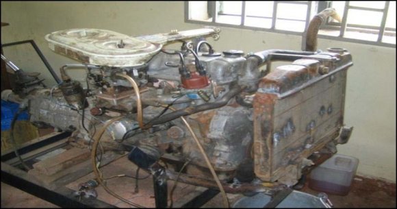
While in Table 2, we list the absolute error e between the true and measured values of a parameter, and we evaluate the relative error er as well. As can be seen from Table 2, our algorithms are able to achieve good accuracy. The absolute errors e of radius are less than 0.10mm, and the relative errors er are less than 0.5%. 8c) is the vector graph of the car engine by our algorithms; it is edited and perfected in AutoCAD2008. In this experiment, a threshold is set for determining whether the closed graphic element is circle. As observed in Fig. (8c), setting the threshold is 0.7, our algorithms not only detect these four large circles correctly, but also fit them with good accuracy. The sizes of circles are marked in AutoCAD2008. Nevertheless, the small circles and slight contours can't be detected completely. If we decrease the threshold value appropriately, these small circles and slight contours will be detected. But the vectorization accuracy may be dropped. Furthermore, several small circles are also detected and fitted correctly. Notice that the left isolated circle, which has the inner and outer concentric contours, is detected correctly. Also, the line contour can be fitted with ideal precision. However, Fig. (9c) also shows the limitation of our algorithms in the slight and complicated details of image. The circle with diameter of 16.55mm is nonexistent, it should not be found. And some contours are not with respect to the original contours ideally. For instance, the circular arc is represented by the irregular arc segments and curves. The following work will aim to resolve these problems.
8. CONCLUSIONS
In this paper, an algorithm for sub-pixel edge detecting based on facet model is adopted for the preprocessed industrial CT image. For the obtained contour, we can calculatethe parameters of circle using the improved fast algorithm based on probability of existence map. Then, a set intersection algorithm of fitting a straight line is applied for recognizing the line. Finally, use the perpendicular bisector tracing algorithm and the least squares function to recognize circular arc. Thus, a vectorization system of industrial CT image is designed, which provides the platform for our experiments. Experimental results show indeed that our algorithms are capable of recognizing the circle, line and circular arc with an excellent accuracy. Furthermore, the vectorization performance for the whole image is preferable. It can satisfy the industrial CT image vectorization requirements of higher precision, rapid speed and non-contact. In the future, we will focus on extending this work by recognizing the relative complex graphic elements as ellipse, regular polygon.
9. VII.
V ( a )


| Number | Circle Center | Radius | Radius | Pe |
| (pixel) | (pixel) | (mm) | ||
| 1 | (430, 576) | 27.798 | 13.860 | 0.867 |
| 2 | (520, 538) | 28.452 | 14.186 | 0.919 |
| 3 | (573, 455) | 29.520 | 14.718 | 0.908 |
| 4 | (578, 360) | 30.635 | 15.274 | 0.774 |
| 5 | (540, 264) | 32.172 | 16.040 | 0.870 |
| 6 | (440, 219) | 35.642 | 17.770 | 0.785 |
| 7 | (320, 233) | 36.254 | 18.076 | 0.847 |
| 8 | (246, 333) | 37.170 | 18.533 | 0.729 |
| 9 | (237, 445) | 40.871 | 20.378 | 0.841 |
| 10 | (314, 547) | 42.133 | 21.007 | 0.877 |