1. I. Introduction
he boundary element method [1,2] is a helpful tool to solve the problems of computational mechanics. Many researchers and scientists use standard BEM, with the boundary approximation done by using linear segments (boundary elements), or standard BEM is improved by considering the conditions of a given problem [1][2][3][4][5][6][7][8][9][10][11][12][13][14][15][16][17][18][19]. The advantage of using linear boundary elements is the opportunity to analytically calculate the integrals, while with curvilinear elements generally, it is possible to do numerical integration [20].
The boundary element method, in particular, the fictitious load method formulated to solve the boundary value and boundary-contact problems of elasticity for a circular ring and its parts are improved in the present paper if considering that the circular segment of the boundary is divided into arcs instead of linear segments. This allows to describe the considered area more accurately and to arrive at a more accurate solution of the problem. So, when the considered area is limited with circles or their parts, i.e., with the coordinate axes of the polar coordinate system, then by dividing the circle into small arcs, we can formulate BEM in the polar coordinate system with all integrals solved analytically. In particular, a fictitious load method is considered in the polar coordinate system, whereas it was described in a Cartesian coordinate system by Crouch and Star field [1].
The article gives a fundamental solution written down in polar coordinate systems serving as a basis to obtain a numerical solution, and a problem of constant forces distributed along the arc is considered. A numerical procedure is presented and boundary coefficients of influence are written out. Two test boundary-contact problems are solved: 1. Elastic equilibrium of an infinite area with a circular hole is studied when a circular ring inserts near the hole; normal constant stress is given on the internal surface of the ring, the body is free from stresses in the infinity, and the conditions of continuity of displacements and stresses are given on the contact line. Numerical values are obtained by using: a) analytical solution, b) standard BEM, i.e., when a circular boundary divides into linear segments, and c) PCSBEM, i.e., when the boundary divides into arcs, and the results obtained in all three cases are compared to one another. 2. A boundary-contact problem is solved for a doublelayer circular ring when the internal circular boundary is loaded with a normal variable force, the outer boundary is not loaded, and conditions of a rigid contact are given for the contact line. The numerical results are obtained by using standard BEM and PCSBEM and are compared to one another. MATLAB software was used to obtain the relevant numerical values and graphs for both problems.
2. II. The Fundamental Solution in the Cartesian Coordinate System
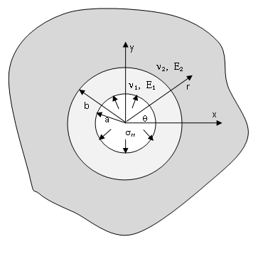
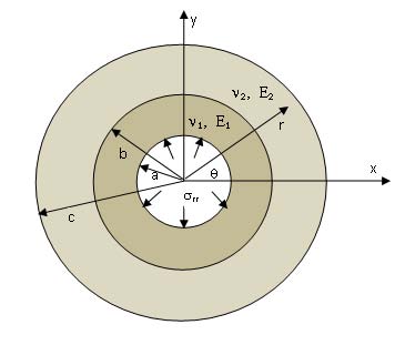
Let us consider the problem shown in The solution to this problem is given by the following function [1]:
where ? is the Poisson's ratio. The displacements will be written down as follows:
where
( ) ? + = 1 2 E Gis shear modulus, and E is Young's modulus.
For the plane deformation, the stresses for Kelvin's problem will be written down as follows:
( ) ( ) [ ]( ) ( ) ( ) [ ] ( ) ( ) [ ] ( )[ ] . 2 1 2 1 , 1 2 2 , 21 2 , , , , , , , , , , , , , xy xyg g F xg g F y x yg g F xg g F yg g F xg g F y x ? ? + ? ? = ? ? + ? = ? + ? ? = ? ? ? ? ? ? ? ? ?As it can be seen from ( 1), (3), the stress at point 0 , 0 = = y x has the singularity. It can be shown that these stresses correspond to the point force at the origin of coordinates [21].
For the sake of simplicity, we mean that ( )
y x i F F F , =force is applied to the origin of coordinates.
3. III. The Fundamental Solution in the Polar Coordinate System
Let us write down formulae (1), ( 2) and (3) in [22]. Following certain algebraic transformations, we obtain the following expression for the function ( )
polar coordinate system ? , r ( ) ? ? 2 0 , 0 < ? ? < ? ry x g , : ( ) ( ) ( ) . ln 1 4 1 , , 1 r r g y x g ? ? ? ? ? = ?For the components of a displacement vector, we will obtain the following equations:
( ) ( ) [ ] ( ) ( ) ( ) ( ) [ ] sin 4 3 2 cos 2 , ~, sin 2 cos 4 3 2 , ~, 1 1 , 1 , 1 , 1 1 y y y x y x y x x x g r g G F g r G F r u g r G F g r g G F r u ? ? ? ? ? ? ? ? ? ? + ? = ? + ? ? =and for the components of the stress tensor we will obtain:
( ) ( ) [ ] ( ) ( ) ( ) ( ) [ ] ( ) ( ) [ ] ( ) [ ], sin 2 1 cos 2 1 , ~ , sin 1 2 cos 2 , ~, sin 2 cos 1 2 , ~, 1 , 1 , 1, 1 , 1 , 1 , 1 , 1 , 1 , 1 , 1 ,g r g F g r g F r g r g F g r g F r g r g F g r g F r ? ? ? ? ? ? ? ? ? ? ? ? ? ? ? ? ? ? ? ? + ? ? = ? ? + ? = ? + ? ? = ( ) ( ) ( ) , ln 1 4 1 , 2 2 y x y x g + ? ? = ? ?? ? ? ? ? ? ? ? ? ? ? ? ? ? ? ? = ? ? = ? = ? ? = ? ? =By using the superposition principle, we can solve the problem for an infinite elastic body, with a set of point forces acting at any of its points. If distributing such forces continuously along some line of the plane, we will obtain a problem with the forces given along this line.
4. IV. Constant Forces Distributed the Curve
Let us consider the following problem: constant
( ) ( )( ) ( ) [ { ( ) ( ) ( ) ( ) ( )] ( ) ( ) ( ) ( )} ( ) ( ) ( ) ( ) ( ) ( ) { ( )( ) [ ( ) ( ) ( ) ( ) ( ) ( )]},2 1 2 1 2 1 2 2 1 2 1 2 1 2 1 2 ? ? ? ? ? ? ? ? ? ? ? ? ? ? ? ? ? ? ? ? ? ? ? ? ? ? ? ? ? ? ? ? ? ? ? + ? + ? ? ? + ? ? ? ? ? = ? ? ? ? ? + ? + ? + ? ? ? = r P P G r u P r P G( ) ( ) ( ) ( ) ( ) [ { ( ) ( ) ( ) ( ) ( ) ( ) ( ) ( ) ( ) [ ( ) ( ) ( ) ( ) ( ) ( ) ( ) ( ) ( ) ( ) [ { ( ) ( ) ( ) ( ) ( ) ( ) ( ) ( ) ( ) [ ( ) ( ) ( ) ( ) ( )( ) ( ) ( ) ( ) ( ) [ ( ) ( ) ( ) ( ) ( ) ( ) ( ) ( ) ( ) [ ( ) ( ) ( ) ( ) () . 6) and ( 7) are displacements and stresses in an infinite elastic body when constant
2 1 2 1 2 1 2 1 2 1 2 1 2 1 2 1 2 1 2 1 2 1 2 1 ? ? ? ? ? ? ? ? ? ? ? ? ? ? + ? ? ? ? ? ? + ? ? ? ? ? ? = ? ? ? ? ? ? ? ? ? + ? ? ? ? ? ? ? ? ? ? ? + ? ? ? ? ? ? = ? ? ? ? ? ? ? ? ? ? ? ? ? ? ? ? ? ? ? ? ? ? ? ? ? ? ? ? = ? ? ? ? ? ? ? ? ? ? ? ? ? ? ? ? ? ? ? ? ? ? ? ? ? ? ? ? ? ? ? ? ? ? ? ? ? ? ? ? ? ? ? ? ? ? ? ? ? ? ? ? ? ? ? ? ? ? ? ? ? ? ? ? ? ?r r P t = and ? ? P t = forces are applied to 2 1 ? ? ? ? ?arc of a circle with the radius r . These equations are the basis for the boundary element method considered later. The following peculiarity of the analytical solution given above is worth mentioning. Displacements from the origin of coordinates to the infinitely distanced points are not limited because of the logarithm included in them. Therefore, equations (6) show only relative displacements. In any concrete case, we must choose a reference point and determine the displacement in respect of such a point.
5. V. Numerical Procedure
The analytical solution obtained above is the basis for the boundary element method used to obtain a numerical solution of the boundary value problem of the theory of elasticity. Let us explain the physical aspect of this method by using a specific example. Let us consider a boundary value problem for an infinite body with a hole (with a circular hole in our case). We will consider a plane deformation. Let us denote the boundary of the cut, which is a circle in our case, by C (See Fig. 3). At any point of the C curve, local s and n coordinates have the direction of a tangent and its perpendicular. Therefore, they change at different points along the border. We take these coordinates so that the direction of n should coincide with the direction of an outer normal at the same point as the border and s should coincide with the direction of the boundary line. In this case, the direction of the boundary line is anticlockwise. Let us assume that the same normal stress ( the whole length of every element, and the tangent is free from stress. In this case, the boundary conditions will be as follows:
( ). , 1 , 0 , N i p i s i n ? = = ? = ? ?Let us imagine that constant normal and tangent stresses act on every element of the circle, e.g., let us denote the normal and tangent stresses acting on the element j by j n P and j s P , respectively.
It should be noted that the real normal and tangent tresses acting on the element j do not equal to j n P and j s P , if stresses act on other elements, too.
Therefore, there are two different kinds of stresses for every element. For example, for the element j , we have applied stresses ) applied to the element j .
By considering the boundary conditions, we will obtain the following equations: It should be noted that j n P and j s P stresses in these equations are fictitious values. They are introduced as an intermediate quantity to obtain the numerical value of the problem, and they have no physical essence. However, a linear combination of a fictitious load presented with formulae (8) has a physical essence in the considered problem, and is the basis to obtain a system of algebraic equations (9). After solving this system, we can express displacements and stresses at any point in a body with another combination of j n P and j s P , ( N j ? , 1 =
) fictitious load.
The above-described boundary element method is called a fictitious load method [1].
6. VI. Influence Coefficients
Let us write down the expressions of the tangent and normal displacements and stresses in the middle point of the i -th element caused by fictitious loads j n P and j s P , N j ? , 1 = applied to the j -th element. For the displacements, we will have: wher e r and ? are coordinates in the local coordinate system, with its center coinciding with the middle point of the i -th element. Generally, the displacements and stresses in the i -th element are functions of the j s P and j n P fictitious load on all N elements. So, by (10) and (11), we can write down: 10) and (11). For example, the ij sn A coefficient is calculated with the expression given in curly braces at j n P of the first equation of (10).
( ) ( )( ) ( ) [ ( ) ( ) ( ) ( )]} ( ) ( ) ( ) ( ) ( ) [ ] ( ) ( ) ( ) ( ) ( ) [ ]( ) ( )( ) ( ) [ ( ) ( ) ( ) ( ) ( )]}2 1 2 1 2 1 2 2 1 2 2 1 2 2 1 2 1 2 1 2 ? ? ? ? ? ? ? ? ? ? ? ? ? ? ? ? ? ? ? ? ? ? ? ? ? ? ? ? ? ? ? ? ? ? ? ? ? ? ? ? ? ? ? ? ? ? + ? ? ? ? ? ? ? ? ? ? ? = ? ? ? ? ? ? ? ? ? ? ? + ? ? ? + ? ? ? ? + ? ? ? =) ( ) ( ) ( ) ( ) [ ( ) ( ) ( ) ( ) ( ) ( ) ( ) ( ) ( ) ( ) [ ( ) ( ) ( ) ( ) ( ) ( ) ( ) ( ) ( ) ( ) [ ( ) ( ) ( ) ( ) ( ) ( ) ( ) ( ) ( ) ( ) [ ( ) ( ) ( ) ( ) ( ) ( ) ( ) ( ) ( ) ( ) [ ( ) ( ) ( ) () ( ) ( ) ( ) ( ) ( ) ( ) [ ( ) ( ) ( ) ( ) ( ) , 32 1 2 1 2 1 2 1 2 1 2 1 2 1 2 1 2 1 2 1 2 1 2 1 ? ? ? ? ? ? ? ? ? + ? ? ? ? ? ? ? ? + ? ? ? ? ? ? ? ? ? + ? ? ? ? ? ? ? ? ? = ? ? ? ? ? ? ? ? ? ? ? ? ? ? ? ? ? ? ? + ? ? ? ? ? ? ? ? ? + ? ? ? ? ? ? ? ? ? = ? ? ? ? ? ? ? ? ? ? ? ? ? ? ? ? ? ? + ? ? ? ? ? ? ? ? ? ? ? ? ? ? ? ? ? ? ? = ? ? ? ? ? ? ? ? ? ? ? ? ? ? ? ? ? ? ? ? ? ? ? ? ? ? ? ? ? ? ? ? ? ? ? ? ? ? ? ? ? ? ? ? ? ? ? ? ? ? ? ? ? ? ? ? ? ? ? ? ? ? ? ? ? ? ? ? ?( ) ( ) , ,1 1 ? ?7. VII. Numerical Examples and Discussion
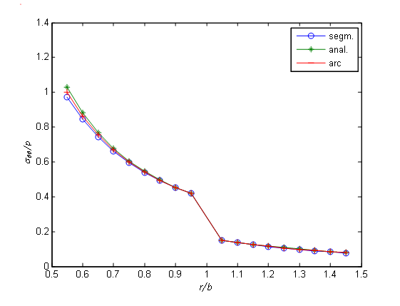
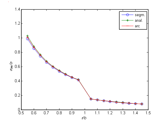
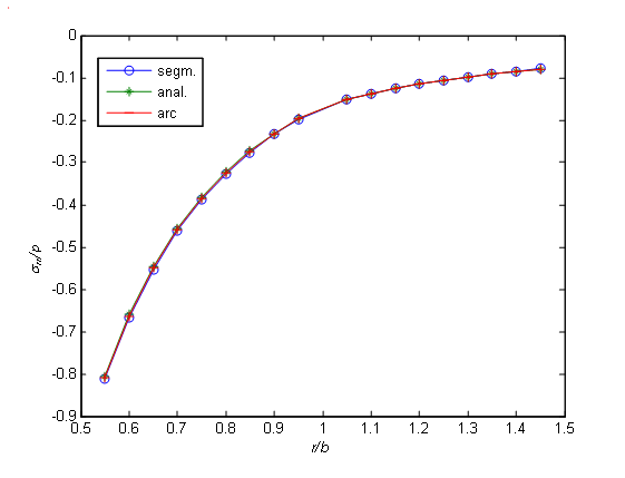
There are two test problems of using a fictitious load method given below. We have an exact solution to one problem. Therefore, in the case of dividing the boundary into segments and arcs, the numerical results obtained by using the boundary element method will be compared to the exact values. Another problem will compare the numerical values obtained by using the fictitious load method to one another in case of dividing the boundary into segments on the one hand and into arcs on the other hand. and for the stresses, the expressions will be as follows: E as its elastic characteristics (See Fig. 4). p rr ? = ? normal stress is given on the internal surface of the ring, while in the infinity, the body is free from stresses, and the continuity conditions of displacements and stresses are given on b r = contact surface. So, we will have the following boundary conditions:
( ) ( ) ( ) ( ) ( ) ( ) ( ) ( ) . , , , : 2 1 2 1 2 1 2 1 ? ? ? ? ? ? ? ? u u u u b r r r r r rr rr ? = ? = = = =The solution to this problem is obtained from standard formulae [23,24] for a thick-wall cylinder. In particular, the radial and tangential stresses are calculated with the following formulae [1]: surface are divided into n=90 elements each, and the obtained visual and numerical results are presented in Fig. 5, Fig. 6, Table 1 and Table 2, while in cases shown in Fig. 7, Fig. 8, Table 3 and Table 4, they are divided into 180 elements each. 9. This problem, too, is symmetrical to both coordinate axes and therefore, we will consider it for a one-fourth of a circular ring. So, the area to be considered is
2 1 ? + ? = ? ,where ? ? ? ? ? ? ? ? ? ? = ? 2 0 , 1 ? ? b r a , ? ? ? ? ? ? ? ? ? ? = ? 2 0 , 2 ? ? c r b .The boundary conditions will be written down as follows: The conditions of a rigid contact will be written down as follows: 2, when n=90 and Fig. 8, Table 4, when n=180), is almost twice as less in terms of percents. It should be noted that in case of dividing the boundary into very small elements, e.g., when n=180, the error is more, as the arithmetic operations with very small numbers results in additional errors (counter error).
( ) ( ) ( ) ( ) ( ) ( ) ( ) ( ) . , , , :Paragraph 7.2 considers the boundary-contact problem for a double-layer circular ring with a normal
8. VIII. Conclusion
The article develops BEM, in particular, the fictitious load method in the polar coordinate system (PCSBEM) to solve the boundary value and boundarycontact problems of the theory of elasticity for the areas limited by the coordinate axes of a polar coordinate system. The bodies relevant to such areas are quite frequent in practice, e.g., in building the underground structures (tunnels), in mechanical engineering, etc. Consequently, the above-described method (PCSBEM) is one of the means to obtain the adjusted solutions of the problems of computational mechanics, as the boundary of the considered area is divided not into small segments, like in case of a standard boundary element method (BEM), but into small arcs. In this case, the boundary of the considered area can be described more accurately, and consequently, the solution to the problem will be more accurate. To illustrate this case, two test boundary-contact problems are solved by using standard BEM and PCSBEM. The obtained numerical results given as tables and graphs are analyzed in paragraph 7. 5, where one can see that they coincide with one another quite exactly.
![Fig. one known as Kelvin's problem of plane deformation [1]. Year 2018 J © 2018 Global Journals Development of Boundary Element Method in Polar Coordinate System for Elasticity Problems . 1 are a line of the point force applied along axis z in the infinite elastic plane.](https://engineeringresearch.org/index.php/GJRE/article/download/1861/version/100979/2-Development-of-Boundary_html/21419/image-2.png)


| ? | ?? | / | p | in the ring | 5 . 0 | ? | b r | ? | 1 | and infinite body | b r | ? | 1 | (n=90) | ||||
| Approximate solution | Relative error, percent | |||||||||||||||||
| No. | r / | b | Exact solution | In case of the division into segments | In case of the division into arcs | Segments | Arcs | |||||||||||
| 1 | 0.5500 | 1.0294 | 0.9726 | 1.0010 | 5.5160 | 2.7574 | ||||||||||||
| 2 | 0.6000 | 0.8827 | 0.8446 | 0.8637 | 4.3169 | 2.1543 | ||||||||||||
| 3 | 0.6500 | 0.7686 | 0.7437 | 0.7561 | 3.2348 | 1.6174 | ||||||||||||
| 4 | 0.7000 | 0.6780 | 0.6621 | 0.6701 | 2.3412 | 1.1706 | ||||||||||||
| 5 | 0.7500 | 0.6049 | 0.5950 | 0.6000 | 1.6392 | 0.8196 | ||||||||||||
| 6 | 0.8000 | 0.5451 | 0.5392 | 0.5422 | 1.0956 | 0.5478 | ||||||||||||
| 7 | 08500 | 0.4956 | 0.4923 | 0.4939 | 0.6601 | 0.3300 | ||||||||||||
| 8 | 0.9000 | 0.4540 | 0.4528 | 0.4534 | 0.2769 | 0.1395 | ||||||||||||
| 9 | 0.9500 | 0.4189 | 0.4194 | 0.4191 | 0.1096 | 0.0548 | ||||||||||||
| 10 | 1.0500 | 0.1512 | 0.1507 | 0.1509 | 0.3242 | 0.1621 | ||||||||||||
| 11 | 1.1000 | 0.1377 | 0.1370 | 0.1374 | 0.5607 | 0.2803 | ||||||||||||
| 12 | 1.1500 | 0.1260 | 0.1250 | 0.1255 | 0.7963 | 0.3981 | ||||||||||||
| 13 | 1.2000 | 0.1157 | 0.1146 | 0.1151 | 1.0238 | 0.5119 | ||||||||||||
| 14 | 1.2500 | 0.1067 | 0.1053 | 0.1060 | 1.2381 | 0.6192 | ||||||||||||
| 15 | 1.3000 | 0.0986 | 0.0972 | 0.0979 | 1.4361 | 0.7181 | ||||||||||||
| 16 | 1.3500 | 0.0914 | 0.0900 | 0.0907 | 1.6165 | 0.8083 | ||||||||||||
| 17 | 1.4000 | 0.0850 | 0.0835 | 0.0843 | 1.7787 | 0.8894 | ||||||||||||
| 18 | 1.4500 | 0.0793 | 0.0777 | 0.0785 | 1.9234 | 0.9714 | ||||||||||||
| Average | 1.6605 | 0.8306 | ||||||||||||||||
| ? | rr / | p | in the ring |
| ? | ?? | / | p | in the ring | 5 . 0 | ? | b r | ? | 1 | and infinite body | b r | ? | 1 | (n=180) | ||||
| Approximate solution | Relative error, percent | |||||||||||||||||
| No. | r / | b | Exact solution | In case of the division into segments | In case of the division into arcs | Segments | Arcs | |||||||||||
| 1 | 0.5500 | 1.0294 | 0.9895 | 1.0095 | 3.8708 | 1.9317 | ||||||||||||
| 2 | 0.6000 | 0.8827 | 0.8539 | 0.8683 | 3.2648 | 1.6331 | ||||||||||||
| 3 | 0.6500 | 0.7686 | 0.7475 | 0.7580 | 2.7475 | 1.3757 | ||||||||||||
| 4 | 0.7000 | 0.6780 | 0.6622 | 0.6701 | 2.3276 | 1.1659 | ||||||||||||
| 5 | 0.7500 | 0.6049 | 0.5960 | 0.6005 | 1.4713 | 0.7274 | ||||||||||||
| 6 | 0.8000 | 0.5451 | 0.5400 | 0.5445 | 0.9356 | 0.1101 | ||||||||||||
| 7 | 08500 | 0.4956 | 0.4930 | 0.4940 | 0.5246 | 0.3228 | ||||||||||||
| 8 | 0.9000 | 0.4540 | 0.4531 | 0.4536 | 0.1982 | 0.0881 | ||||||||||||
| 9 | 0.9500 | 0.4189 | 0.4183 | 0.4185 | 0.1432 | 0.0955 | ||||||||||||
| 10 | 1.0500 | 0.1512 | 0.1509 | 0.1510 | 0.1984 | 0.1323 | ||||||||||||
| 11 | 1.1000 | 0.1377 | 0.1372 | 0.1375 | 0.3631 | 0.1452 | ||||||||||||
| 12 | 1.1500 | 0.1260 | 0.1252 | 0.1256 | 0.6349 | 0.3175 | ||||||||||||
| 13 | 1.2000 | 0.1157 | 0.1150 | 0.1154 | 0.6050 | 0.2593 | ||||||||||||
| 14 | 1.2500 | 0.1067 | 0.1058 | 0.1062 | 0.8435 | 0.4686 | ||||||||||||
| 15 | 1.3000 | 0.0986 | 0.0978 | 0.0983 | 0.3043 | 0.8114 | ||||||||||||
| 16 | 1.3500 | 0.0914 | 0.0907 | 0.0912 | 0.7659 | 0.2188 | ||||||||||||
| 17 | 1.4000 | 0.0850 | 0.0844 | 0.0847 | 0.7059 | 0.2353 | ||||||||||||
| 18 | 1.4500 | 0.0793 | 0.0788 | 0.0791 | 0.6305 | 0.2522 | ||||||||||||
| Average | 1.1408 | 0.5717 | ||||||||||||||||
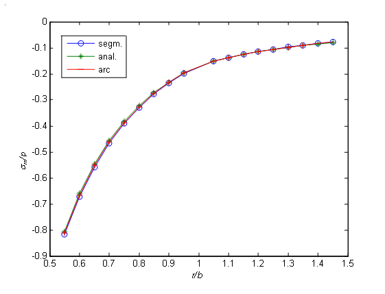
| ? | rr / | p | in the ring | 5 . 0 | ? | b r | ? | 1 | and infinite body | b r | ? | 1 | (n=180) | |||
| Approximate solution | Relative error, percent | |||||||||||||||
| No. | r / | b | Exact solution | In case of the division into segments | In case of the division into arcs | Segments | Arcs | |||||||||
| 1 | 0.5500 | -0.8072 | -0.8124 | -0.8098 | 0.6519 | 0.3268 | ||||||||||
| 2 | 0.6000 | -0.6605 | -0.6675 | -0.6640 | 1.0552 | 0.5308 | ||||||||||
| 3 | 0.6500 | -0.5464 | -0.5535 | -0.5499 | 1.3036 | 0.6496 | ||||||||||
| 4 | 0.7000 | -0.4558 | -0.4622 | -0.4590 | 1.4077 | 0.7060 | ||||||||||
| 5 | 0.7500 | -0.3827 | -0.3880 | -0.3854 | 1.3926 | 0.7013 | ||||||||||
| 6 | 0.8000 | -0.3229 | -0.3271 | -0.3250 | 1.2871 | 0.6452 | ||||||||||
| 7 | 08500 | -0.2734 | -0.2764 | -0.2749 | 1.1177 | 0.5647 | ||||||||||
| 8 | 0.9000 | -0.2318 | -0.2339 | -0.2329 | 0.9077 | 0.4640 | ||||||||||
| 9 | 0.9500 | -0.1967 | -0.1980 | -0.1973 | 0.6761 | 0.3173 | ||||||||||
| 10 | 1.0500 | -0.1512 | -0.1522 | -0.1517 | 0.6921 | 0.3496 | ||||||||||
| 11 | 1.1000 | -0.1377 | -0.1383 | -0.1380 | 0.4447 | 0.1880 | ||||||||||
| 12 | 1.1500 | -0.1260 | -0.1263 | -0.1262 | 0.2216 | 0.1397 | ||||||||||
| 13 | 1.2000 | -0.1157 | -0.1158 | -0.1158 | 0.0207 | 0.0512 | ||||||||||
| 14 | 1.2500 | -0.1067 | -0.1065 | -0.1066 | 0.1600 | 0.0625 | ||||||||||
| 15 | 1.3000 | -0.0986 | -0.0983 | -0.0985 | 0.3226 | 0.1210 | ||||||||||
| 16 | 1.3500 | -0.0914 | -0.0910 | -0.0912 | 0.4690 | 0.2728 | ||||||||||
| 17 | 1.4000 | -0.0850 | -0.08.45 | -0.0848 | 0.6011 | 0.2752 | ||||||||||
| 18 | 1.4500 | -0.0793 | -0.0787 | -0.0790 | 0.7203 | 0.3415 | ||||||||||
| Average | 0.7473 | 0.3726 | ||||||||||||||
| b) Double-layer circular ring | ||||||||||||||||
| Let us consider the boundary-contact problem | ||||||||||||||||
| shown in Fig. | ||||||||||||||||
| ? on the circle | r = | a |