1. I. INTRODUCTION
he Speech recognition in recent times has proved it's' efficacy in all our day to day activities, its' almost invading our lives, every individual has directly or indirectly has interaction with it. It's built into our mobile phones, game consoles, smart watches and all Digital Signal processing machines. It is the tool we use to interact with robots, though it's not a new field of endeavor, it has been around for decades, but the field is gaining acceptance and recognition in present times. There is need for Engineers and Technologists to embrace this technology for accurate Speech recognition in certain environments. Speech recognition accuracy lies in the bosom of deep learning, which makes it possible to predict accurately with almost 95% confidence when we interact with computers. This is achieved simply in this research by feeding the sound recording into the neural network and training it to produce the text and the owner of the voice. The research also intends to look into certain difficulties encountered when designing a system that recognizes speech since certain factors; such as the speed in speeches, which determines the mode of speaking and it varies from human to human [1], the research will try to examine this by using some kinds of extraction and processing techniques in addition to the deep learning neural network. In the study conducted by Vibha Tiwari, he examined that the property of speech signal can change as a function of time, and he used the MFCC extraction method to study the properties of signals such as energy, zero crossing, and correlation [1]. In a similar research on voice recognition algorithm using MFCC by Lindasalwa et.al, it was established that human voice conveys much information such as gender, emotion, and identity of the speaker, the research then used the tool of MFCC techniques to solve the problem of recognition which is based on human hearing perceptions that is limited to 1kHz. The MFCC was then used to study the variations of the human ears' critical bandwidth [2].
2. II. Methodology
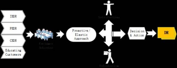
The model was designed for the purpose of recognising when a particular speaker is on board, so that other participants in a meeting can listen to the contributions of that particular speaker, the algorithm is also designed to recognise the country where the speaker is from, since each country from the meeting has been coded with a particular frequency range which is unique to that particular speaker. Immediately after his or her contributions, the deep learning can now give access to the others for their contributions, thereby acting as a multiplexer, giving access at a time during the speech and denying others for a while.
3. a) The Coding procedures
The current speaker making a speech is recognized by the machine as having a high value which is coded with digit 1, while as at that time the other speeches from the prospective Speakers are regarded as low value, with code 0, that is the speech of an accessed Speaker is given a priority as high value, while others are given low values and the machine will deny them an access.
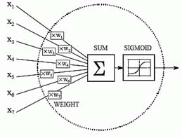
The network Architecture assumed a continuous variable of vocabulary size. The soft computing aspect of the system involves; Speech recognition algorithm, Neural network building and integration of program segments. The system is coded using python functional programming language. The neural network used is a four layered neurons with two separate hidden layers of order 9 and 6 respectively before the output. The neural training employed is back propagation algorithm, to ensure that errors are computed through the sigmoid functions and brought to the barest minimum to recognize a speech.
4. c) The Model Conception
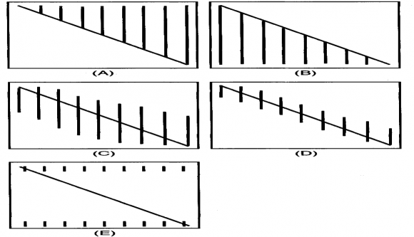
The research tries to model a speech recognition system using the properties of a sine wave and the energy values relating to the amplitudes of the wave. The system used the efficacy of Fast Fourier transforms to obtain the Spectrogram which contains the full sound clip. The results from the energy equivalent 2 2A E = were introduced into the neural network to carry out the machine learning processes in other to give an output which is to recognise what the speaker is trying to say and the speaker. The Speech recognition algorithm was design using the MFCC extraction techniques which is based on human hearing perception. The amplitude of a wave is related to the energy which it transports; longer wavelength means that there is lesser energy, but the low frequency waves have wider T (period), while the high frequency waves have lower period, this can be viewed from the energy wave diagram below. A wave is an energy transport medium which transports energy along a medium without transporting matter. The amount of energy carried by a wave is related to the amplitude of the wave and directly proportional to the square of amplitude, this property has been used to generate the Spectrogram, which shows the amount of energy absorbed and contributed by each number in the pitch of the audio signal recorded.
5. d) The Coding Procedure for the Algorithm
The speech recognition system algorithm is designed using a four layer neural network with four input neurons and a bias which is attached to each layer. The variable 1 X (size of the vocabulary) which is divided into small words i.e. 2-100words with weight of 0.70, medium words ranging from 100-1000 words with weight .25 and large words ranging from at least 10,000 words with weight 0.05. The un-forbidden code for recognising a small word is (100) the small words is coded with digit 1, while medium words and large words are coded with 0 respectively for this system to recognize the speech spoken in this research. The variable representing the second neuron is 2 X (Channel characteristics) is divided into low, medium and high with weights 0.05, .25 and 0.70 respectively for the neurons to recognize whether the channel is okay for the . The last bias is always assi9gned with digit value 1. The back-propagation algorithm ensures that the input data is repeatedly presented to the neural network in the training process. In each presentation the output of the neural network is compared to the desired output while the error is computed to see whether the neurons are actually predicting the speech. This error is then fed back to the neural network and is used to adjust the weights such that the error decreases with each cycle of the training and the neural model gets closer and closer to producing the desired output of the speech recognition.
The coding procedures as they are fed into the algorithm can be selected according to the following rules, 1 , , , , in the sequence one. It's worth noting that the last digit in all the cases is the bias, which is always digit 1. This is the way they have been supplied to the code in the python deep learning algorithm designed for this research.
6. e) Neural Architecture
The voice recognition system used in this research assumes the pattern of recurrent neural network, which conforms to the below architecture, but in actual sense of this research, four inputs have been used and the two separate hidden layers of the order of nine and six neurons in the middle preceding the output. They are many factors responsible for speech recognition of sound wave, but the most important four have been focused for the purpose of the research. The fifth neurons are the bias to make it a non-linear model, for easier recognitions speeches using the intelligent deep learning of neuron-computing. The processing neurons in the first and second hidden layers ensure that the threshold energy values in the spectrum are intelligently interpreted with accuracy in speed because they are tightly connected for faster information delivery to the output neurons.
For the purpose of this research, the training algorithm has been coded in python algorithmic language and the training was repeated with 250epoch to minimize the errors and getting a better output, which matched the threshold values in all the cases.
The Neural network model using the XOR data is repeatedly presented to the neural network.
At each presentation, the error between the network inputs, the hidden layers and the desired output were calculated, which is the threshold energy value when it has been activated through the sigmoid function. The computed values are then fed back to the neural network for proper adjustments. These sequences of events were done repeated until an acceptable error has been reached, when the network no longer appears to be learning, and the final output computed.
7. III. The Speech Recognition Principles
The following procedures were adopted for the speech recognition machine to fully act as an automatic speech recognizer; in other to fully develop an automatic speech recognition algorithm, the first step is to record an Audio signal from microphone, and store it in a file, thereafter sampling is carried out to select the portion of appreciable size, this is done using various sampling theorem, since sound waves are recorded as a continuous signals of varying amplitude, there is need to convert it into a discrete time signal in other make representation in digital form easier. The next step after this is to carry out the Fourier Transformation (FT) and Fast Fourier Transform (FFT), the extraction of the Audio signal is necessary in other to obtain the energy equivalent of the digitized signal which can be fed into neural Algorithm for deep learning to take and speech recognition to be achieved. These processes are discussed as a separate segment below.
8. a) The Sampling Method
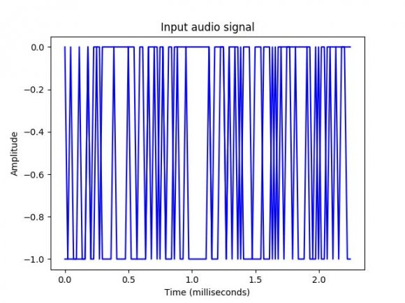
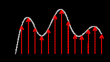
Sampling can be defined as the acquisition of a continuous signal at a discreet time interval, since sound signal travel as waves an in one-dimensional plane. At every moment in time, they have a single value based on the height of the wave. For the purpose of this research a complex Audio signal of sampling size of 44,100Hz is assumed. The ideal sampling function , where T is the sampling interval. A typical sound waves recorded can be viewed to have a complex structure like figure 1, but it involves thousands of wave forms, because of this, there is need to convert this to discreet time signal and convert it into numbers and bits to make easier for representation, this can be viewed in the figures 2 and 3 below. In this research, for speech recognition, a sampling rate of 16 kHz (16,000 samples per second) is enough to cover the frequency range of human speech in other to completely design an automatic speech recognition system.
9. Sampled segment of the Speech
In other to turn this signal into numbers, there is need to record the maximum displacement at equally spaced points through the sampling process, which is shown in the figure 4.
By taking the a reading thousands of times a second and recording a number of the sound wave at that point in time, as in this research where a sampling size of 16000 samples per second enabled the machine to fully recognize the speech. To correct the errors in gaps, the research used NYQUIST theorem, which made it possible to perfectly reconstruct the original sound waves from the spaced out samples, as long as the Nyquist requirements are met; max 2w w s ? . After the sampling, there is need to carry out some processing on Audio data by grouping the sampled Audio into 20 milliseconds long, this makes extraction easier on sample.
The principles employed in this research involves converting the time domain signals into the frequency domain, and understanding its' frequency components using the mathematical tool of Fourier transform. This is important because it gives a lot of information about the sound signal in question. This is the most powerful mathematical tool invented to characterise signals through transformation from time domain to frequency domain. The FFT has been used effectively by [4], [6] to recognise the voice of some physically challenged people who can only use their voices to register and attend examination. [ ]
) ( * ) ( ) ( * ) ( ) ( w X w H t X t h FFT w Y ? = ,The mathematical complexities of this principles have been taken care of using commands in the python libraries of version 27X If X (w), H (w) and Y (w) are the Fourier Transform of X (t), H (t) and Y (t) respectively [2] This is the most useful tool when it comes to building a speech recognition system; it finds a useful application in converting our signals from the time domain to frequency domain. Since the signal must be converted into usable forms of features vector, which includes extraction techniques such as; MFCC, PLP, PLP-RASTA etc. The Mel Frequency Ceptral Coefficient is a powerful tool that has been used by many researchers to extract unique features of human voice. It is based on linear cosine transform of the log power spectrum on the non-linear Mel frequency scale, because of the equally spaced of the frequency band which make it possible to approximate human voice; it is useful in carrying out extraction of unique features [1], [3]. The expression
) 100 1 ( log 2595 10 f m + = is usedto convert the normal frequency f to the Mel scale m. The advantage of the MFCC is that it relates to the energy absorbed in terms velocity and acceleration of the speech [2], [4].
The extraction process can be viewed as the means of separating the complex sound wave into its' components parts, since some of the notes are low pitched, next lower pitched and so on. The procedures of mathematical tool used are the efficacy of Fourier transform which breaks apart the complex sound wave into simpler forms making it up. By this method it is easier to measure the energy value of each pitch of frequency band.
It is not easy to recognise a complex sound wave by the neural network, but these difficulties can be overcome by breaking it down into components parts making it up in other to obtain the equivalent energy relating to the pitch of frequency band.
10. IV. Results And Discussion
11. a) Analysis of Visualizing the Audio Signal
The speech recognition analysis actually started from the recording of the Audio signal through a microphone as input the device; thereafter the recorded Audio signal is stored in a wave file. The processes of sampling commences as it has been described in the previous segment of this research, the python 2.7X was used to carry out the sampling at certain frequency and conversion into discreet form to obtain the numerical values using the following line of commands; import numpy as np import matplotlib.pyplot as plt from scipy.io import wavfile
The above command lines read from the file while the path is provided by the using the command; frequency_sampling, audio_signal = wavfile. read ("hello.wav"), this will return two values that's the sampling frequency and the Audio values.
It is important to display the parameters like sampling frequency of the audio signal, data type of signal and its duration, by using the commands; print('\nSignal shape:', audio_signal.shape) print('Signal Datatype:', audio_signal.dtype) print('Signal duration:', round(audio_signal.shape[0] / float(frequency_sampling), 2), 'seconds'), with these the normalisation of the signal can be done easily by invoking the command; audio_signal = audio_signal / np.power (2,15). In this research for simplicity, the first 100 values were extracted to visualise the signal using the commands;
12. show()
This can be seen in the figure5. This is the an output graph and data extracted for the above audio signal as shown in the image here
![It was used to analyse spectrum to continuous signals where it was discovered that it was the faster mathematical method that eliminates redundancy in terms of signals which do not contain needed information. If given N sample size in time domain, and it is required to operate this in frequency domain; to convert each frame of N samples from time domain into frequency domain. The Fourier Transform is to convert the convolution of the glottal pulse U[n] and the vocal tract impulse response H[n] in the time domain. The mathematical representation of this statement can be expressed by the equation below:](https://engineeringresearch.org/index.php/GJRE/article/download/1849/version/100973/2-Deep-Learning-Algorithm_html/21321/image-5.png)
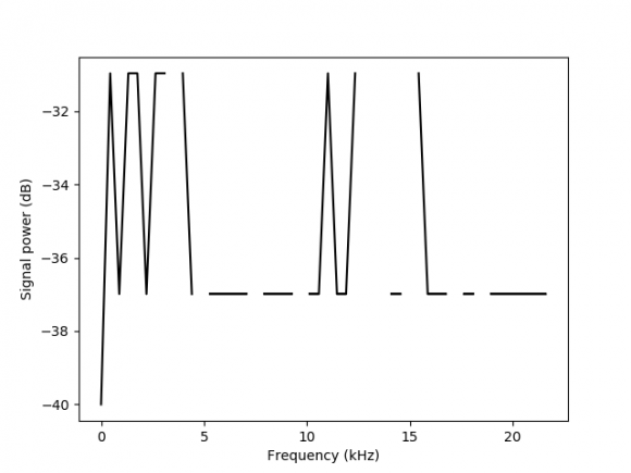
![audio_signal = audio_signal [:100] time_axis = 1000 * np.arange(0, len(audio_signal), 1) / float(frequency_sampling plt.figure() plt.plot(x_axis, signal_power, color='black') plt.xlabel('Frequency (kHz)') plt.ylabel('Signal power (dB)') plt.](https://engineeringresearch.org/index.php/GJRE/article/download/1849/version/100973/2-Deep-Learning-Algorithm_html/21323/image-7.png)