1. I. Introduction
Dr. Louay S. Yousuf in order to avoid of the exible cam mechanism of stable and dangerous working velocities. Cveticanin, [4]. described the mathematical model of cam-follower mechanism with two coupled non-linear, ordinary second-order differential equation. He developed new criteria for designing the cam profile based on the stable motion. Gue et al, [5]. applied the Fourier spectrum tool on cam acceleration based on frequency domain. The dynamic response at low frequency range has been related to different cam rotational speeds such as (700, 900, and 1100) rpm. Hsu and Pisano, [6]. Investigated the simulation of contact forces at three different speeds (660, 1650, and 2500) rpm of a finger-follower cam system. They determined the contact position between the cam and the follower by using the constrained equation method. The force at low speeds is employed to derive the dynamic Coulomb friction coefficients at contact points. chew and chuang, [7]. Implemented the generalized Lagrange multiplier method of camfollower systems over a range of cam speeds. The results are checked by using a second approach of nonlinear programming technique. Fabien et-al, [8]. Explained a linear quadratic optimal control theory to design a high-speed of Dwell-Rise-Dwell (D-R-D) cams. Three approaches of D-R-D cam design are presented. In the first approach, the cam designed to be optimal at a fixed operating speed. In the second approach, the cam profile is determined by minimizing the sum of quadratic cost function over a range of discrete speeds. The third technique uses trajectory sensitivity minimization to design a cam which is insensitive to speed variations. Jiang et-al, [9]. Formulated the problems of minimizing vibrations in high-speed camfollower systems over a range of speeds (800-3600) rpm. A universal Hermite cam displacement is suggested. Alzate et-al, [10] detected the sudden transition to chaos in a radial cam and a at faced follower. They observed that the follower detaches from the cam under the variation of cam rotational speeds. Yan et-al, [11]. Derived the equation of motion for a cam-follower system by using variable cam-input angular velocity. They found that peak values of follower output motion have been decreased by using proper cam-input trajectories. Bagci and Kurnool, [12]. Presented a Fourier series-Laplace transform to find the follower response at any time and at any cycle. They cam is a mechanical device which is used to transmit the motion to the follower. The proposed cam can be used in motor car camshafts to operate the engine valves. Recently, much research effort has been spent to study the contact-impact problem. UNLUSOY and TUMER, [1]. derived the exact quasi-linear solution to represent the non-linear behavior of cam mechanism at different cam speeds. The critical examination of the simulation has been made by using the equivalent viscous damper instead of Coulomb friction model. Hamidzadeh and Dehghani, [2]. used Hill's infinite determinant method to present a solution of linear, second-order, ordinary differential equation for different rotational speeds. They found that the system is stable for low values of cam rotational speeds. A few unstable regions are occurred when the speed is increased gradually. The effect of both operational speed and damping on the dynamic stability has been determined. Tounsi et-al, [3] presented the multiple scales method to resolve the equation of motion unstable regimes. They calculated the instability regions A II. Simulation Procedure measured the critical cam speeds and follower jump conditions. Many researches have been done to reveal the effect of Lyapunov exponents on human-gait locomotion. The aim of this paper is to implement Lyapunov analyses to characterize stability of nonlinear dynamic.
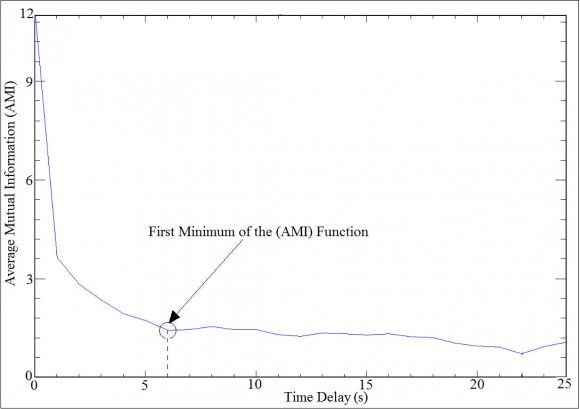
Time delay (T) and the embedding dimension (dE) are necessary for the nonlinear analysis. A computer algorithms was carried out to calculate the time delay and the embedding dimension. Time delay is an integer number between two samples from time series. If the time series represent a continuous on with samples taken every t seconds, then the delay parameter may be expressed as, [16]:
Where, a = 1.7508 (N), b = 0.038 N/mm. The first term (a) represents the initial preload to avoid follower jumping during high speeds. The second term (b) represents the spring force varying with each position of the follower motion. The contact force is defined as:
The impact parameters that used in the Solidworks simulation are indicated in Table 1.
? -- -- -- --The local dynamic stability of a cam-follower is quantifed by calculating Lyapunov exponent values. Maximum finite-time Lyapunov Exponents were calculated based on the algorithm published by Rosenstein et al. [14]. The dynamic analysis was constructed by using the data of follower displacement. A valid state space is any vector space containing a suficient number of independent coordinates, [15]. An appropriate state space can be reconstructed from a single time series as in the equation below:
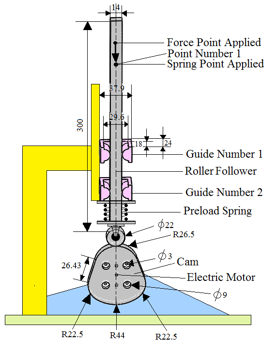
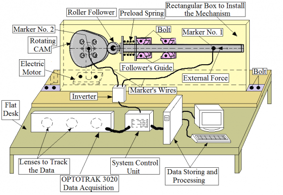
The cam, roller-follower, and guides are designed in a Solid Works program using the experimental dimensions of existing mechanisms, [13]. A simulation was carried out for the planar case using the block commands. The general dimensions of the cam, follower, and its guides are measured in (mm) and are shown in Fig. 1. Different follower guide's clearances such as C = 0.3, 0.5, 1, 1.5, and 2 mm have been used in the simulations. Fig. 2 shows the clearance between ( follower and its guide. The follower with clearance has three degrees of freedom translation in x, y directions and rotation about z axis. A marker has been stick on the follower by choosing a suitable point, which has the coordinates (x: 0, y: 272 mm, z: 0), as indicated in
2. IV. Experimental Setup
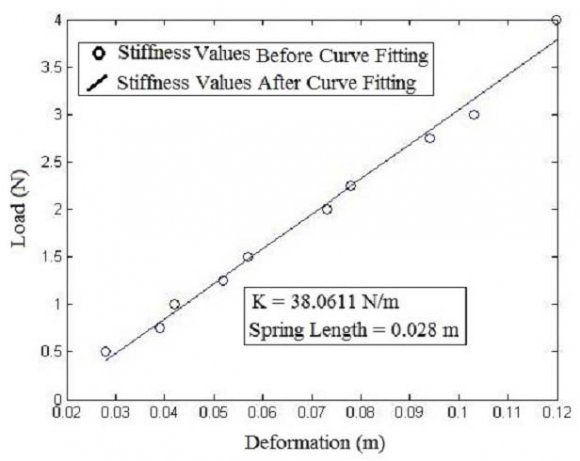
Our rig is based on a radial cam with an oscillating roller-follower. A spring with the elastic constant is used to maintain the contact between the cam and the follower. Figure 5 shows the curve fitting of spring stiffness values. With non-periodic systems and large value of successive delay coordinates may become causally unrelated, and the reconstruction is no longer representative of the true dynamics, [16]. A related difficulty with attractor reconstruction involves the choice of dE. The embedding dimension is the algorithm which determines the global number of a space data vectors. It converts a single time series into a multidimensional object in an embedding space vectors. dE is usually estimated greater than twice the topological dimension (m) as:
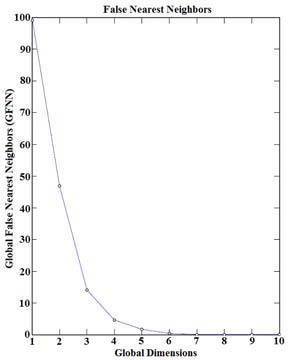
Embedding dimension was computed from a Global False Nearest Neighbors (GFNN) algorithm. GFNN compares the distances between neighboring trajectories in the reconstructed state space at successively higher dimensions, as illustrated in Fig. 4.
3. Figure 5: Load-Deflection Curve Fitting
The global dimension is chosen where the total percentage of false neighbors approaches zero, thus providing a suffcient number of coordinates to define the system state at all points in time, [17]. It can be suggested that it may be more appropriate to ? w the reconstruction window, ? w , rather than ? alone, in which ? w and ? are interchanged as dictated by the particular context, as illustrated below: [18,19,20,21]: The stiffness of the contact-retaining spring is determined to cause a minimum force pushing the follower system towards the cam. The system with follower's guide clearance C = 0.3 mm was used. The cam-follower mechanism has been manufactured by a 3D printing filament technique device. The mechanical device was shown to be appropriately coupled to electronic systems for the acquisition, storage and processing of experimental data, [10]. The main feature of the experimental set-up can be summarized as follows: (1) The cam motion was controlled by a brush-less motor driven through an embedded controller. The angular position of the cam and the driving motor were assumed to be identical. (2) The measures of the cam and the follower positions are obtained through highresolution optical encoders (markers). The marker has been stick on the follower which has the coordinates (x: 0, y: 272 mm, z: 0). (3) The OPTOTRAK / 3020 used to capture the motion through an infrared 3-D camera. The signals are analyzed using MATLAB program. The experimental rig was depicted in Fig. 6.
Lyapunov exponents quantify the average exponential rate of divergence of neighboring trajectories in state space domain, and thus provide a direct measure of the sensitivity of the system to infinitesimal perturbations [15]. The maximum Lyapunov exponent ( ) can be defined by using the equation below:
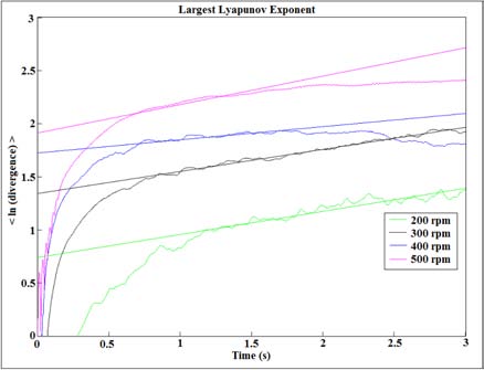
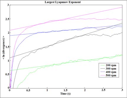
The Rosenstein method [14] estimates the largest Lyapunov exponents of a reconstructed attractor. The input to the program is a scalar follower displacement along with several parameters such as time delay and embedding dimension. The basic principle of this algorithm is to calculate the diverging ratio between trajectories in the state space domain, [22,23]. The largest Lyapunov exponent was estimated from best-fit linear slopes of these local divergence ?
The Lyapunov exponent values were estimated from the slopes of linear fits to curves defined by: curves. The average local Lyapunov exponents determine the stability of the dynamic system using attractor trajectories. When the attractor is non-periodic, the trajectories diverge, on average, at an exponential rate characterized by the largest Lyapunov exponent [24]. The presence of a positive exponent is sufficient for diagnosing chaos and represents local instability in a particular direction. Larger values of Lyapunov exponents imply more divergence and variability of a system while smaller values reect less divergence and variability. On the other hand, the lower positive Lyapunov exponents imply less sensitivity to perturbations. [25].
4. VI. Results and Discussion
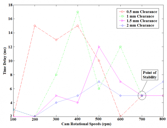
Table (2) shows the simulation of Lyapunov exponent values varying with cam rotational speeds and follower guides' clearances. It can be observed that the largest Lyapunov exponent values are extremely constant for cam rotational speed N = 200 rpm and N = 500 rpm. The system with lowest Lyapunov exponent gives indication of local dynamic stability. The system with largest Lyapunov exponent represents the dynamic instability. The system with follower guide's clearance C = 2 mm and cam rotational speed N = 300 rpm has largest Lyapunov exponent. The system with follower guide's clearance C = 1.5 mm and cam speeds N = 400 rpm represents the local dynamic stability.
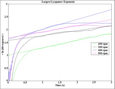
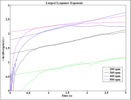
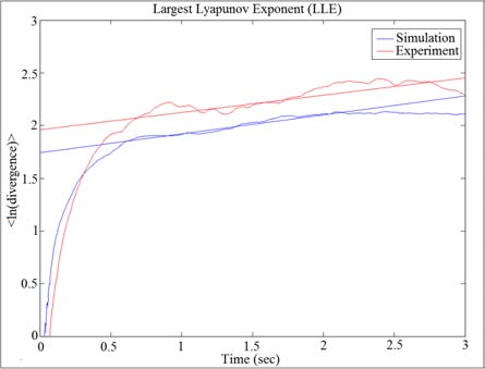
The verification of the follower linear displacement based on experiment and simulation techniques has been shown in Fig. 7. The simulation results were carried out using the y-direction because the simulation was obvious and clear. The verification was done by using N = 400 rpm of cam rotational speed. The system with follower's guide clearance C = 0.3 mm was used in the verification. In high-speed machinery, the jump is a situation where the cam and follower substantially scattered.
5. VII. Conclusions
Table (3) shows the large Lyapunov exponent values verification varying with cam rotational speeds. The system with followers guide clearance C = 0.3 mm was used in the verification. The system with cam speed Î?"t: Discrete time steps.
The system with follower guide's clearance C = 2 mm and cam rotational speed N = 300 rpm has largest Lyapunov exponent. The system with follower guide's clearance C = 1.5 mm and cam speeds N = 400 rpm represents the local dynamic stability. The average logarithmic divergence curve has been oscillated around the straight line of curve fitting experimentally. In the simulation analysis, the average ?:
![) = [x(t), x(t + T ), x(t + 2T ), ...., x(t + (d E ? 1)T ? = T ?t )] Effect of Local Dynamic Stability of a Ploydyne Cam with Translated Follower on Lyapunov Exponent Parameter over a Range of Speeds F = a ? b ? F c = K? n + ?? n ?](https://engineeringresearch.org/index.php/GJRE/article/download/1814/version/101450/4-Effect-of-Local-Dynamic_html/31161/image-3.png)
![d(t) = De ?t y(i) = 1 ?t ln[d j (i)]Effect of Local Dynamic Stability of a Ploydyne Cam with Translated Follower on Lyapunov Exponent Parameter over a Range of Speeds](https://engineeringresearch.org/index.php/GJRE/article/download/1814/version/101450/4-Effect-of-Local-Dynamic_html/31166/image-8.png)
| Simulation Parameters | ||
| Parameter's Definition | Value | Unit |
| Kinematic Sliding Velocity | 10.16 | mm/s |
| Kinematic Coefficient of Friction | 0.2 | |
| Static Sliding Velocity | 0.1 | mm/s |
| Static Coefficient of Friction | 0.3 | |
| Contact Bodies Stifiness | 1100049.92 | N/mm |
| Exponent | 2 | |
| Max Damping | 0.58839681 | N/(mm/s) |
| Penetration | 0.1 | mm |
| Frame Per Second | 500 | |
| Cam Speed (rpm) | Clearance (0.5mm) | Clearance (1 mn) | Clearance (1.5 mm) | Clearance (2 mm) |
| 200 | 0.284 | 0.211 | 0.217 | 0.181 |
| 300 | 0.192 | 0.28 | 0.208 | 0.416 |
| 400 | 0.384 | 0.321 | 0.124 | 0.128 |
| 500 | 0.239 | 0.191 | 0.267 | 0.277 |
| 600 | 0.348 | 0.369 | 0.203 | 0.179 |
| 700 | 0.241 | 0.266 | 0.307 | 0.283 |
| 800 | 0.236 | 0.3 | 0.366 | 0.349 |
| Carm Speed (rpm) | Simulation | Experiment | Error % |
| 340 | 0.18 | 0.164 | 8.88 |
| 385 | 0.431 | 0.454 | 5.06 |
| 410 | 0.244 | 0.210 | 13.93 |
| 423 | 0.26 | 0.299 | 13.04 |