1. Introduction
ptimization is a work of achieving the best result under given limitation or constraints. Now a day, optimization is used in all the fields like construction, manufacturing, controlling, decision making, prediction etc. The final target is always to get feasible solution with minimum use of resources. In this field computers make a revolutionary impact on every field as it provides the facility of virtual testing of all parameters that are involved in a particular design with less involvement of human efforts, benefits in less time consuming, human efforts and wealth as well.
Today we use computer-aided design where a designer designs a virtual system on computer and gives only command to test all parameters involved in that design without even the need for a single prototype.
A designer only to design and simulate a system and set all the parameter limitation for the computer.
Computer-aided design technique becomes more effective with the additional feature of autogeneration of solutions after it's mathematically formulation of any system or design problem. Auto generation of solution, this feature is come into nature with the development of algorithms. In past years, real world designing problems are solved by gradient descent optimization algorithms. In gradient descent optimization algorithm, the solution of mathematically formulated problem is achieved by obtaining its derivative. This technique is suffered from local minima stagnation [1,2] more time consuming and their solution is highly dependent on their initial solution.
The next stage of development of optimization algorithms is population basedstochastic algorithms.These algorithms had number of solutions at a time so embedded with a unique feature of local minima avoidance. Later population based algorithms are developed to solve single objective at a time either it may be maximization or minimization on accordance the problems objective function. Some popular algorithms for single objective problems are Moth-Flame optimizer (MFO) [3], Bat algorithm (BA) [4], Particle swarm optimization (PSO) [5], Ant colony optimization (ACO) [6], Genetic algorithm (GA) [7], Cuckoo search (CS) [8], Mine blast algorithm (MBA) [9], Krill Herd (KH) [10], Interior search algorithm (ISA) [11] etc. These algorithms have capabilities to handle uncertainties [12], local minima [13], misleading global solutions [14], better constraints handling [15] etc. To overcome these difficulties different algorithms are enabled with different powerful operators. As mention above here is only objective then it is easy to measure the performance in terms of speed, accuracy, efficiency etc. with the simple operational operators.
In general, real world problems are nonlinear and multi-objective in nature.In multi-objective problem there may be some objectives are consisting of maximization function while some are minimization function. So now a day, multi-objective algorithms are in firm attention.
Let's take an example of buying a car, so we have many objectives in mind like speed, cost, comfort level, space for number of people riding, average fuel consumption, pick up time required to gain particular speed, type of fuel requirement either it is diesel driven, petrol driven or both etc. To simply understand multiobjective problem, from Fig. 1, we considertwo objectives, first cost and second comfort level. So we go for sole objective of minimum cost possible then we have to deny comfort level objective and vice-versa. It means real word problems are with conflicting objectives. So as, we are disabled to find an optimal solution like single objective problems. About multiobjective algorithm and its working is detailed described in next portion of the article. The No free launch [16] theorem that logically proves that none of the only algorithm exists equally efficient for all engineering problem. This is the main reason that it allows all researcher either to propose new algorithm or improve the existing ones. This paper proposed the multi-objective version of the well-known whale optimization algorithm(WOA) [17]. In this paper non-sorted WOA (NSWOA) is tested on the standard unconstraint and constrainttest function along with some well-known engineering design problem, their results are also compared with contemporary multi-objective algorithms Multi objective Colliding Bodies Optimizer (MOCBO) [18], Multi objective Particle Swarm Optimizer (MOPSO) [19][20], Non-dominated Sorting Genetic Algorithm (NSGA) [21][22][23], non-dominated sorting genetic algorithm II (NSGA-II) [24] and Multi objective Symbiotic Organism Search (MOSOS) [25] that are widely accepted due to their ability to solve real world problem.
The structure of the paper can be given as follows: -Section 2 consists of literature; Section 3 includes the proposed novel NSWOAalgorithm; Section 4 consists of competitive results analysis of standard test functions as well as engineering design problem and section 5 includes real world application, finally conclusion based on results and future scope of work is drawn.
2. II.
3. Literature Review
As the name describes, multi-objective optimization handlessimultaneously multiple objectives. Mathematically minimize/maximize optimization problem can be written as follows:
/ : ( ?) = { ( ?),(? ? , = 1,2, . . . ,
Where q is the number of inequality constraints, r is the number of equality constraints,k is the number of variables, is the i th inequality constraints, no is the number of objective functions, indicates the i th equality constraints, and [ , ] are the boundaries of i th variable.
Obviously, relational operators are ineffective in comparing solutions with respect to multiple objectives. The most common operator in the literate is Pareto optimal dominances, which is defined as follows for minimization problems:
where ? = ( , , ? , ) and ? = ( , , ? , ). For maximization problems, Pareto optimal dominance is defined as follows:
where ? = ( , , ? , ) and ? = ( , , ? , ).
These equationsshow that a solution is better than another in a multi-objective search space if it is equal in all objective and better in at least one of the objectives. Pareto optimal dominance is denoted with ? and ?. With these two operator's solutions can be easily compared and differentiated.
Population based multi-objective algorithm's solution consists of multiple solution. But with multiobjective algorithm we cannot exactly determine the optimal solution because each solution is bounded by other objectives or we can say there is always conflict between other objectives. So the main function of stochastic/population based multi-objective algorithm is to find out best trade-offs between the objectives, so called Pareto optimally set [26][27][28].
The principle of working for an ideal multiobjective optimization algorithm is as shown in Fig. 2.
Step No. -1 Find maximum number of nondominated solution according to objective, it expresses the number of Pareto optimal set so as shows higher coverage
Step No. -2 Choose one of the Pareto optimal solution using crowding distance mechanism that fulfills the objectives.
4. F
Now a day recently proposed sole objective algorithms are equipped with powerful operators to provide them a capability to solve multi-objective problems as well. In the same manner we proposed NSWOA algorithm in a hope that it will perform efficiently for multi-objective problems. These are: Multi-objective GWO [29], Multi-objective Bat Algorithm [30], Multiobjective Bee Algorithm [31],Pareto Archived Evolution Strategy (PAES) [32], Pareto-frontier Differential Evolution (PDE) [33], Multi-Objective Evolutionary Algorithm based on Decomposition (MOEA/D) [34], Strength-Pareto Evolutionary Algorithm (SPEA) [35,36]andMulti-objective water cycle algorithm with unconstraint and constraint standard test functions [37] [38].Performance measurement for approximate robustness to Pareto front of multi-objective optimization algorithms in terms of coverage, convergence and success metrics.
The computational complexity of NSWOA algorithm is order of ( )where N is the number of individuals in the population and M is the number of objectives. The complexity for other good algorithms in this field: NSGA-II, MOPSO, SPEA2 and PAES are (
). However, the computational complexity is much better than some of the algorithms such as NSGA and SPEA which are of ( ).
5. III.
Non-Dominated Sorting Whale Optimization Algorithm (nswoa) The Whale Optimization Algorithm (WOA) with sole objective was proposed by Mirjalili Seyedali and Andrew Lewis in 2016 [17]. It is basically a stochastic population based, nature inspired algorithm. In this algorithm the basic strategy based on special hunting nature of humpback whales.Some fact about humpback whales that they are: fancy creatures, biggest mammals in the world and have power of think, learn, judge, communicate, being emotional etc. They are also considered as predators as they never sleep, only half of the brain sleeps, as they have to breathe from surface of the ocean. One more interesting fact about whales is their hunting or foraging behavior to hunt small fishes. Such type of foraging behavior is known as bubble-net feeding strategy where whales went down in water approximate 10-15 meter and then after start to produce bubbles in a spiral shape encircles prey and then follows the bubbles and moves upward the surface. This foraging behavior is done by making distinct bubbles along with a circle or '9-shaped path' represented in Fig. 3 . *( )
( ) D C X t X t ? ? ?? ?? ? (1) ( 1) *( ) . X t X t A D ? ? ? ?? ? ?? ? ?? ?? (2)2 * A a r a ? ? ?? ? ? (3) 2* C r ? ?? (4)Where: ? is a variable linearly decrease from 2 to 0 over the course of iteration and r is a random number [0, 1].
6. b) Bubble-net attacking method
In order to mathematical equation for bubblenet behaviour of humpback whales, two methods are modelled as:
7. i. Shrinking Encircling Mechanism
This technique is employed by decreasing linearly the value of a ? from 2 to 0. Random value for vector ? in rang between [-1, 1].
8. ii. Spiral Updating Position
Mathematical spiral equation for position update between humpback whale and prey that was helix-shaped movement given as follows:
(
? ? ? ? ? ? ? ? ? ? ? ? ? ? ? ? ? ?? ? ?? ?? ?? ? ??? ?? ?(6)Where: p expresses random number between [0, 1].
iii. Search for prey
9. A
10. ??
Vector can be used for exploration to search for prey;
vector A ?? also takes the values greater than one or less than -1. Exploration follows two conditions
. rand D C X X ? ? ?? ?? ?????? ?? ? (7)( 1).
rand X t X A D ? ? ? ?? ? ?????? ?? ??(8)Finally follows these conditions: ? Position of whales are updated as a spiral or helix shaped movement function and so as value of next position of whales is decided ? The value of absolute distance is achieved which is basically a distance between the current best solution (whales current position) to the final (prey position) optimal solution ? We assume that there is 50-50% probability that whale either follow the shrinking encircling or logarithmic path during optimizationmuch needed to update their position towards optimal one ? Stage 3 ? Termination counter in integrated to limit/forcefully stop the search in uncertain search space (max. iteration counter to forcefully converge the search to optimal one) ? Size of the position vector matrix is continuously reduced over the course of iteration due to directed search to find global best solution ? Continuously position of the whalesis updated towards the optimal one viaeither follow the shrinking encircling or logarithmic path during optimizationequation for each iteration ? Likewise, multi-objective optimization the NSWOA algorithm is made to capable to store the pareto
? 1 A ? ??11. ? Stage4
Note: We assume that there is 50-50% probability that whale either follow the shrinking encircling or logarithmic path during optimization. Mathematically we modelled as follows:
Global Journal of Researches in Engineering ( ) Volume XVII Issue IV Version I optimal solutions in a collectionset and make it as flexible to change solution over the course of iteration ? Solution is assigned a rank according to their ability as if a solution is not dominated by other solution is assigned rank1, dominated by only solution assigned rank 2 and so on & if collection set is full (archive size) over predefined size then some solutions that are less non-dominated (according to fitness value) in natureare directed to be out from the collection set according to the crowding distance mechanism. This collection set is similar to the term achieve used in MOSOS and NSGA-II. It is a repository to store the best non-dominated solutions obtained so far. The search mechanism in NSWOA is very similar to that of WOA algorithm, in which solutions are improved using position vectors. Due to the existence of multiple best solutions, however, the best whales position should be chosen from the collection set.
In order to select solutions from the archive to establish tunnels between solutions, we employ a leader selection mechanism. In this approach, the crowding distance between each solution in the archive is first selection and the number of solutions in the neighbourhood is counted as the measure of coverage or diversity. We require the NSWOAalgorithm to select solutions from the less populated regions of the archive using the following equation to improve the distribution of solutions in the archive across all objectives.
This section proposes multi-objective version of the WOA algorithm called NSWOA algorithm. The nondominated sorting has been of the most popular and efficient techniques in the literature of multi-objective optimization. As its name implies, non-dominated sorting sort Pareto optimal solutions based on the domination level and give them a rank. This means that the solutions that are not dominated by any solutions is assigned with rank 1, the solutions that are dominated by only one solution are assigned rank 2, the solutions that are dominated by only two solutions are assigned rank 3, and so on. Afterwards, solutions are chosen to improve the quality of the population base on their rank. The better rank, the higher probability to be chosen. The main drawback of non-dominated sorting is its computational cost, which has been resolved in NSGA-II.
The success of the NSGA-II algorithm is an evidence of the merits of non-dominated sorting in the field of multi-objective optimization. This motivated our attempts to employ this outstanding operator to design another multi-objective version of the WOA algorithm. In the NSWOA algorithm, solutions are updated with the same equations presented in equation 3.9. In every This mechanism allows better solutions to contribute in improving the solutions in the population. It should be noted that non-dominated sorting gives a probability to dominated solutions to be selected as well, which improves the exploration of the NSWOA algorithm. Flow chart of NSWOA algorithm is represented as Fig. 4.
12. Constraint Handling Approach
With the extended literature survey we find that the population based algorithms are the common way to solve the multi-objective problems as they are more commonly provides the global solution and capable of handling both continuous and combinational optimization problem with a very high coverage and convergence. Multi-objective problems are subjected to various type of constraints like linear, non-linear, equality, inequality etc. So with these problems embedded it is very difficult to find simple and good strategy to achieve considerable solutions in the acceptable criterion. So in this paper NSWOA algorithm uses a very simple approach to get feasible solutions. In this mechanism, after generating number of solutions at each generation, all the desirable constraint checked and then some solution that fulfills the criterion of acceptable solution are selected and collected them in achieve. Afterward non dominated solutions added in archive as we find more suitable solution to get acceptable solution. So as if achieve is full then less dominated solutions are removed. Finally, according to crowing distance mechanism all these solutions (more suitable position of the whales) from archive is selected to get desired solution.
13. ?P?_i=c??Rank?_i
(3.9)
iteration, however, the solutions to have optimal position of whalesare chosen using the following equation:
where c is a constant and should be greater than 1 and ???????? ?? is the rank number of solutions after doing the non-dominated sorting.
14. Results Analysis On Test Functions
For determine the performance of proposed NSWOA algorithm is applied to: ? A set of unconstraint and constraint standard multiobjective test functions ? Tested on well-known engineering design problems ? Non-linear, highly complex practical application known as economic constrained emission dispatch (ECED)
? With and Without stochastic integration of wind power (WP) in the next section ? A simple six-operating generational unit with power demand 1200 MW. (Engineering multiobjective design problem) with distinct characteristics like non-linear, non-convex, discrete pareto fronts and convex etc. are selected to measure the performance of proposed NSWOA algorithm. To deal with real world engineering design problem is really a typical task with unknown search space, in this article we include four different engineering problems are considered and performance is compared with various well known algorithms like MOWCA, NSGA-II, MOPSO, PAES and ?-GA multi-objective algorithms. Each algorithm is separately runs fifteen times and numeric results are listed in tables below. To measure the quality of obtained results we match their coverage of obtained true pare to front with respect to their original or true pare to fronts.
15. Initialize the no. of whales, no. of variable, maximum iterations
For numeric as well as qualitative performance of purposed NSWOA algorithm on various case studies we consider Generational Distance (GD) given by Veldhuizen in 1998 [39]for measuring the deviation of the distance between true pare to front and obtained pare to front, Diversity matric (Î?") also known as matrix of spread to measure the uniformly distribution of nondominated solution given by Deb [24]and Metric of spacing (S) to represent the distribution of nondominated distribution of obtained solutions by purposed algorithm given by Schott [40]. where
shows the Euclidean distance (calculated in the objective space) between the Pareto optimal solution achieved and the nearest true Pareto optimal solution in the reference set, is the total number of achieved Pareto optimal solutions.
Î?" = ? | | ( )where, , are Euclidean distances between extreme solutions in true pareto front and obtained pareto front.
shows the Euclidean distance between each point in true pare to front and obtained pare to front.
and 'd' are the total number of achieved Pareto optimal solutions and averaged distance of all solutions.
16. = ? ( ? ) a) Results on unconstrained test problems
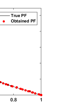
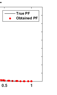
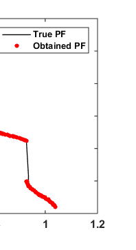
Like as above mentioned, the first set of test problems consist of unconstrained standard test functions. All the standard unconstrained test functions mathematical formulation is shown in Appendix A. Later, the numeric results are represented in Table 1 and best optimal pare to front is shown in Fig. 5.
All the statistical results are shown Table 1 suggests that the NSWOA algorithm effectively outperforms with most of the unconstraint test functions compare to the MOSOS, MOCBO, MOPSO and NSGA-II algorithm. The effectiveness of proposed nondominated version of WOA (NSWOA algorithm) can be seen in the Table 1, represents a greater robustness and accuracy of NSWOA algorithm in terms of mean and standard deviation with the help of GD, diversity matrix along with computational time. However, proposed NSWOA algorithm shows very competitive results in comparison with the MOPSO, MOCBO and MOSOS algorithms and in some cases these algorithms perform better than proposed one. Pare to front obtained by proposed NSWOA algorithm shows almost complete coverage with respect to true pare to front. Year 2017
17. F
The mathematical representation of these performance indicating metric are as follows:
where "d" is the average of all ?? ?? , ?? ?????? is the total number of achieved Pareto optimal solutions, and
?? ?? = min ?? ?|ð??"ð??" 1 ?? (?? ?) ? ð??"ð??" 1 ?? (?? ?)| + |ð??"ð??" 2 ?? (?? ?) ? ð??"ð??" 2 ?? (?? ?)?for all i,j=1,2,?,n. Smallest value of "S" metric gives the global best non-dominated solutions are uniformly distributed, thus if numeric value of ?? ?? and ?? are same then value of "S" metric is equal to zero.
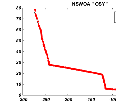
with wind power (ECEDWP). These can be classified into four groups given below: The next set of standard test functions consisting of constrained functions. For constrained test function it should be necessary that NSWOA algorithm has a capability of handling constraints so algorithm is equipped with a death penalty function to search that violate any of the constraints at any level [41]. For comparing the results of different algorithms, we have utilized GD and Î?" metrics. has a capability of handling constraints so algorithm is equipped with a death penalty function to search agents that violate any of the constraints at any level [41]. For comparing the results of different algorithms, we have
18. i. Four-bar truss design problem
The statistical results of four bar truss design problem [42] in given in Table 3 and best optimal front is given in Fig. The statistical results of four bar truss design problem [42] in given in Table 3 and best optimal front is given in Fig. 7. It consists of two minimization objectives displacement and volume with four design control variable mathematically given in Appendix C. Year 2017 F CONST function consists of concave front with linear front, OSY is similar to CONST but consists of many linear regions with different slops while TNK almost similar to wave shaped. These also suggests that NSWOA algorithm has a capability to solve various type of constraint problem. All the constraint test functions are mathematically given in Appendix B.
19. Speed-reducer design problem
The statistical results of speed reducer design problem [43] is given in Table 4 and best optimal front is given in Fig. 8 Pareto optimal front obtained by the NSWOA Algorithm for "Four -bus truss design problem"
The statistical results of speed reducer design problem [43] is given in iii.
20. Welded-beam design problem
The statistical results of welded beam design problem [44] is given in Table 5 and best optimal front is given in Fig. The statistical results of welded beam design problem [44] is given in Table 5 and Table 5: Results of the multi-objective NSWOA algorithms on welded-beam design problem in terms mean and standard deviation
21. Disk brake design problem
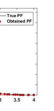
The statistical results of welded beam design problem [44] is given in Table 6 and best optimal front is given in Fig. 10. It is a well-known mechanical design Fig. 10: Paretooptimal front obtained by the NSWOA Algorithm for "Disk brake design problem" Due to high complexity of engineering design problem it is really hard to gain results alike true pare front but we can clearly see that optimal pare obtained by NSWOA algorithm is covers almost whole solutions that are the actual/true solutions of an engineering design problem. From all above tested function we can conclude that problem either it consists of constraints or unconstraint problem NSWOA algorithm shows its capability to solve any kind of linear, non-linear and complex real problem. next section we attached a highly non-linear complex real problem to show its effectiveness regarding the real world complex application with many objectives.
The statistical welded beam design problem [44] is given in Table 6 and best optimal front is known mechanical design problem consists of two minimization objectives stopping time and mass of brake of a disk brake four design control variable mathematically given in Appendix C.
optimal front obtained by the NSWOA Algorithm for "Disk brake design problem"
Due to high complexity of engineering design problem it is really hard to gain results alike true pare to optimal pare to obtained by NSWOA algorithm is covers almost whole solutions that are the actual/true solutions of an engineering design problem. From all above tested function we can conclude that problem either it consists problem NSWOA algorithm shows its capability to solve any kind of linear, linear and complex real world problem. So in the linear complex real problem to show its effectiveness regarding the real ication with many objectives.
22. d) Formulation Of Economic Constrained Emission Dispatch (ECED) With Integration Of (WP) i. Mathematical Formulation Of Wind Power
In case of wind power generation, the output power of wind generator is calculated with the help of a stochastic variable wind speed ? (meter/seconds). Wind speed is a variable function so their probability distribution plays a very important role. Wind sp mathematically formulated as two distribution function, probability density function (PDF) and cumulative distribution function (CDF) as follows:
( ) = ( ) ? ( ) ? * exp ? ( ( ) = 1 ? exp ? ( ) ?, ? 0 objectives stopping time and mass of brake of a disk brake with four design control variable mathematically given in optimal front obtained by the NSWOA Algorithm for "Disk brake design problem"
23. Economic Constrained Emission ) With Integration Of Wind Power Formulation Of Wind Power
In case of wind power generation, the output power of wind generator is calculated with the help of a (meter/seconds). Wind speed is a variable function so their probability distribution plays a very important role. Wind speed mathematically formulated as two-parametric Weibull distribution function, probability density function (PDF) and cumulative distribution function (CDF) as follows: where, S(v) and s(v) are CDF and PDF respectively. Shape factor and scale factor are k and c respectively. The wind speed and output wind power are related as:
) ? , ? 0 (4.1) (4.2)= 0, < ? ? < ? < (4.3)where, and are the rated speed of wind and rated power output. and are cut-out and cut-in speed of wind respectively. The CDF of in the boundary of [0, ] on an accordance with the speed range of wind can be formulated as:
( ) = 1 ? ? 1 + * } + exp [? ( ) ? ], 0 ? < (4.4)Above equation is very meaningful to calculate the ECED problems with speculative wind power with variable speed.
24. ii. Modeling of ECEDWP problem
As power is formulated as system constraint, so the objective function of economic emission dispatch problem (EEDP) stays on unchanged as classical EEDP:
Fuel cost objective is given by:
( ) = ? ( + + ) (4.5)where, the thermal power generators cost coefficients are , , for i-th generator, Sum of the total fuel cost of the system and N is the total number of generators. Total Emission is calculated by:
( ) = ? [{( + + ) * 10 } + * exp ( * )] (4.6)where, , , , and are emission coefficients with valve point effect taking into consideration i-th thermal generator.
25. iii. System Constraints
As wind power generation is considered as system constraint with the summation of stochastic variables the classical power balance constraint changes to fulfill the predefined confidence level.
? ( + ? + ) ? (4.7)where, is confidence level that a power system must follow the load demand and so as it is selected nearer to unity as values lesser than unity represents high operational risk.
represents system losses can be calculated by B-coefficient method given below:
= ? ? + ? + (4.8)So as to change above described power balance constrained equation into deterministic form can be solved as:
{ < + ? ? = ( + ? ? ) ? 1 ? (4.9) + ? ? ? + * ? * (4.10)iv. Reserve capacity system constraint So as to reduce the impact of stochastic wind power on system, up and down spinning reserve needs to be maintained [22]. Such reserve constraints formulated as [15] and [16] respectively:
{? ( ? ) ? + * } ? (4.11) ? ? ? * ( ? ) ? (4.12)where, represents the reserve demand of conventional thermal power plant system and it generally keeps the maximum value of thermal unit, and are maximum and minimum output level of operational generators of i-th unit, and are predefined down and upper confidence level parameter respectively, and are the demand coefficients of up and down spinning reserves.
26. v. Generational capacity constraint
The real output power is bounded by each generators upper and lower bounds given as: ? ? (4.13)
V.
Test System For Economic Emission Dispatch Problem a) 40-Operational Thermal Generating Unit
27. i. Case Study I-40 Thermal-Generator Lossless System Without Wind Power
In this case forty operational generating unit is consider without integration of wind power means all the generating units are coal fired. Input parameters like generators operating limit, fuel cost coefficients and emission coefficients are given in Appendix D and in Table 11. extracted from [45]. System is considered lossless and its solution is compared with three well known multi-objective algorithms like SMODE [45], NSGA-II [45]and MBFA [46] in terms of various objectives such as best cost, best emission and best compromise between both objectives. Best compromise solution is then obtained by the fuzzy based method [47]. Total power demand for this system is 10500 MW. Results obtained by NSWOA algorithm is added to table 7 and best pare to front obtained by NSWOA algorithm is represented in Fig. 12.
Non-Dominated Sorting Whale Optimization Algorithm (NSWOA): A Multi-Objective Optimization Algorithm for Solving Engineering Design Problems
ii. Case study lossless system with wind power All the conditions are remaining same as case study I like input parameters and power demand. While
28. generator lossless system
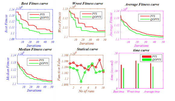
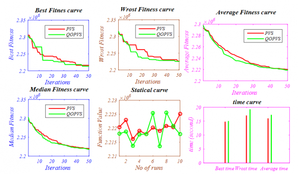
All the conditions are remaining same as case y I like input parameters and power demand. While integrating with wind power plant, the total rated output power of wind farm is set to 1000 MW [45,47].Statistical results obtained by NSWOA algorithm is reported in Table 8 and best optimal front is represented in Fig. 13. integrating with wind power plant, the total rated output power of wind farm is set to 1000 MW [45,47].Statistical results obtained by NSWOA algorithm is reported in sented in Fig. 13. Fig. 13: Pareto optimal front obtained by the NSWOA Algorithm for "40 thermal-generator lossless system with wind power" b) Test system with six operational generating unit This test system consists of six operational generating unit with simply a quadratic fuel and emission objective function for a power demand of 1200 MW. Input data for operational generating unit loading limits and loss parameters are given in Table 12 of Appendix D extracted from [52,53].
29. Be st emission
It is represented in Table 10 that with the objective of least cost objective minimum fuel cost is 6.4197e+04 $ and emission value is 1345.9 lb. But fuel cost increases to 6.992e+04 $ and emission value reduced to a numeric value 1242.7 lb with the objective of emission minimization. Compromise point or true operating point obtained by NSWOA algorithm for multi-objective combined economic emission dispatch (MOCEED) problem is as fuel cost is 6.4830e+04 $ that is higher than minimum fuel cost 6.4197e+04$ and lower than 6.992e+04 $ obtained during least cost and emission value objectives respectively. So as with emission value for true operating point is 1285 lb that is lower than 1345.9 lb and higher than 1242.7 lb obtained during least cost and emission value objectives respectively. Statistical value obtained for compromise point is compared with other techniques solves same MOCEED problem like SPEA2, NSGA-II and PDE in Table 10. Fig. 14 shows 100 non-dominated solutions as true pare to front for 6-opertaional generating for PD=1200 MW.
30. Result Discussion
In almost all the cases that we consider in this article where NSWOA algorithm proves its effectiveness in both prospective quantitative and qualitative. From plots also evident that NSWOA algorithm follows the exact pare to front similar to the true pare to front for all constrained, unconstrained and complex engineering design problem. So as for real world application of economic emission dispatch problem and its integration with stochastic wind power generation. So for this application Wilcox on test (statistical test)is performed.
In Table 9 the signed rank test is presented in third row of each results whereas the calculation time is represented in forth row. For this test null hypothesis cannot be rejected at 5% level for numeric value '0' while null hypothesis is rejected at 5% level with the value of '1'. Where NSWOA algorithm performs superior to other algorithms that are considered for comparative purpose.
NSWOA algorithm shows good performance in both coverage and convergence as main mechanism that guarantee convergence in WOA and NSWO Aalgorithms are continuously shrink its virtual limitation using helix shaped or 9-shaped path strategy in the movement of whales for their random walk. Both mechanism emphasizes convergence and exploitation proportional to maximum number of generation (iteration). Since this complex task might degrade its performance compare to without limitation or free movement should be a concern. However, the numerical results expresses that NSWOA algorithm has a little effect of slow convergence at all. NSWOA algorithm has an advantage of high coverage, which is the result of the selection of position of whales and archive selection procedure. All the position is updated according to their fitness value that enable the algorithm to direct the search space in right direction to find the best solution without trapped in local solution. Archive selection criteria follow all the rules of the entrance and exhaust of any value in it for each iteration and updated when its size full. Solutions of higher fitness in archive have higher probability to thrown away first to improve the coverage of the pare to optimal front obtained during the optimization process.
31. VII.
32. Conclusion
In this paper the non-dominated sorting whale optimization algorithm-multi-objective version of recently proposed whale optimizationalgorithm (WOA) is proposed known as NSWOA algorithm. This paper also utilizes the bubble-net swarming strategy for exploration purpose used in its parent WOA version. The NSWOA algorithm is developed with equipping whale optimization algorithm with crowding distance criterion, an archive and whales position (accordance to ranking) selection method based on Pareto optimal dominance nature. The NSWOA algorithm is first applied on 17 standard test functions (including eight unconstraint, five constraint and four engineering design multi-objective problems) to prove its capability in terms of qualities and quantities showing numerical as well as convergence and coverage of pare to optimal front with respect to true pare to front. Then after NSWOA algorithm is applied to real world complex ECEDWP problem where algorithm proves its dominance over other well recognized contemporary algorithms. The numeric results are stored and represented in performance indices: GD, metric of diversity, metric of spacing and computational time. The qualitative results are reported as convergence and coverage in best pare to optimal front found in 15 independent runs. To check effectiveness of proposed version of algorithm the results are verified with SMODE, MOSOS, MOCBO, MOPSO, NSGA-II and other well recognize algorithms in the field of multi-objective algorithms. We can also conclude from the standard test functions results that NSWOA algorithm is able to find pare to optimal front of any kind of shape. Finally, the result of complex real world ECEDWP problem validates that NSWOA algorithm is capable of solving any kind of non-linear and complex problem with many constraint and unknown search space. Therefore, we conclude that proposed non-dominated version of WOA algorithm has various merits among the contemporary multi-objective algorithms as well as provides an alternative for solving multi or many objective problems.
For future works, it is suggested to test NSWOA algorithm on other real world complex problems. Also, it is worth to investigate and find the best constrained handling technique for this algorithm.
Appendix A: Unconstrained multi-objective test problems utilized in this work.
33. KUR:
Minimize:
ð??"ð??" 1 (??) = ? ?? 10exp (?0.2??? ?? 2 + ?? ??+1 2 ) ? 2 ??=1 ð??"ð??" 2 (??) = ? [|?? ?? | 0.8 + 5??????(?? ?? 3 )] 2 ??=15 5
1 3 i x i ? ? ? ? ? FON: 2 1 1 2 2 1 1 ( ) 1 exp ( ) min 1 ( ) 1 exp ( ) n i i n i i f x x n imize f x x n = = ? ? ? = ? ? ? ? ? ? ? ? ? = ? ? ? ? = ? ? + ? ? ? ? ? ? ? ? 4 4 1 i x i n ? ? ? ? ? ZDT1: ZDT2: Minimise: ?? ?? (??) = ?? ?? Minimise: ð??"ð??" 2 (??) = ð??"ð??"(??) × ??ð??"ð??" 1 (??), ð??"ð??"(??)? ??(??) = 1 + 9 ?? ? 1 ? ?? ?? ?? ??=2 ??ð??"ð??" 1 (??), ð??"ð??"(??)? = 1 ? ? ð??"ð??" 1 (??) ð??"ð??"(??) 0 ? ?? ?? ? 1, 1 ? ?? ?30Where:
Minimise:
ð??"ð??" 1 (??) = ?? 1Minimise: ð??"ð??" 2 (??) = ð??"ð??"(??) × ??ð??"ð??" 1 (??), ð??"ð??"(??)?
Where: SCHN-1 :
??(??) = 1 + 9 ???1 ? ?? ?? ?? ??=2 ??ð??"ð??" 1 (??), ð??"ð??"(??)? = 1 ? ? ð??"ð??" 1 (??) ð??"ð??"(??) ? 2 0 ? ?? ?? ? 1,Minimize: ð??"ð??" 1 (??) = ?? ?? 2 ð??"ð??" 2 (??) = (?? ? 2) 2 A x A ? ? ?Where: value of can be from 10 to 10^5.
34. SCHN-2 :
Minimize:
( ) Where:
1 2 2 x, 1 x 2, 1 3 ( ) 4 x, 3 4 x 4,4( ) 5 if x if x f x if x if x f x x ? ? ? ? ? ? ? < ? ? ? = ? ? ? < ? ? ? ? ? ? > ? ? ? = ? ?ð??"ð??" 1 (??) = ??? 1 2 ? ?? 2 2 + 1 + 0.1??????(16???????????? ? ?? 1 ?? 2 ?) ð??"ð??" 2 (??) = 0.5 ? (?? 1 ? 0.5) 2 ? (?? 2 ? 0.5) 2 0.1 ? ?? 1 ? ??, 0 ? ?? 2 ? ?? BNH:This problem was first proposed by Binh and Korn [48]:
Minimise: ?? ?? (??) = ???? ?? ?? + ???? ?? ?? Minimise: ð??"ð??" 2 (??) = (?? 1 ? 5) 2 + (?? 2 ? 5) 2 ð??"ð??" 1 (??) = (?? 1 ? 5) 2 + ?? 2 2 ? 25 ð??"ð??" 2 (??) = 7.7 ? (?? 1 ? 8) 2 ? (?? 2 + 3) 2 0 ? ?? 1 ? 5,0 ? ?? 2 ? 335. OSY:
The OSY test problem has five separated regions proposed by Osyczka and Kundu [49]. Also, there are six constraints and six design variables.
36. Minimise:
ð??"ð??" 1 (??) = ?? Where:
ð??"ð??" 1 (??) = 2 ? ?? 1 ? ?? 2 ð??"ð??" 2 (??) = ?6 + ?? 1 + ?? 2 ð??"ð??" 3 (??) = ?2 ? ?? 1 + ?? 2 ð??"ð??" 4 (??) = ?2 + ?? 1 ? 3?? 2 ð??"ð??" 5 (??) = ?4 + ?? 4 + (?? 3 ? 3) 2 ð??"ð??" 6 (??) = 4 ? ?? 6 ? (?? 5 ? 3) 2 0 ? ?? 1 ? 10,0 ? ?? 2 ? 10,1 ? ?? 3 ? 5,0 ? ?? 4 ? 6,1 ? ?? 5 ? 5,0 ? ?? 6 ? 10 SRN:The third problem has a continuous Pareto optimal front proposed by Srinivas and Deb [50].
Minimise:
ð??"ð??" 1 (??) = 2 + (?? 1 ? 2) 2 + (?? 2 ? 1) 2 Minimise: ð??"ð??" 2 (??) = 9?? 1 ? (?? 2 ? 1)2Where:
ð??"ð??" 1 (??) = ?? 1 2 + ?? 2 2 ? 255 ð??"ð??" 2 (??) = ?? 1 ? 3?? 2 + 10 ?20 ? ?? 1 ? 20, ?20 ? ?? 2 ?2037. CONSTR:
This problem has a convex Pareto front, and there are two constraints and two design variables.
Minimise:
ð??"ð??" 1 (??) = ?? 1 Minimise: ð??"ð??" 2 (??) = (1 + ?? 2 )/(?? 1 )Where:
ð??"ð??" 1 (??) = 6 ? (?? 2 + 9?? 1 ), ð??"ð??" 2 (??) = 1 + ?? 2 ? 9?? 1 0.1 ? ?? 1 ? 1,0 ? ?? 2 ? 5Appendix C: Constrained multi-objective engineering problems used in this work.
38. Four-bar truss design problem:
The 4-bar truss design problem is a well-known problem in the structural optimisation field [42], in which structural volume (f1) and displacement (f2) of a 4-bar truss should be minimized. As can be seen in the following equations, there are four design variables (x1-x4) related to cross sectional area of members 1, 2, 3, and 4.
39. Minimise:
?? ?? (??) = ?????? * (?? * ??(??) + ð??"ð??"ð??"ð??"ð??"ð??"ð??"ð??"(?? * ??(??)) + ð??"ð??"ð??"ð??"ð??"ð??"ð??"ð??"(??(??)) + ??(??))
Minimise: ð??"ð??" 2 (??) = 0.01 * (? 2 ??(1) ? + ? 2 * ???????? (2) ??(2) ? ? ((2 * ????????(2))/??(3)) + (2/??(1))) 1 ? ?? 1 ? 3,1.4142 ? ?? 2 ? 3,1.4142 ? ?? 3 ? 3,1 ? ?? 4 ? 340. Speed reducer design problem:
The speed reducer design problem is a well-known problem in the area of mechanical engineering [43], in which the weight (f1) and stress (f2) of a speed reducer should be minimized. There are seven design variables: gear face width (x1), teeth module (x2), number of teeth of pinion (x3 integer variable), distance between bearings 1 (x4), distance between bearings 2 (x5), diameter of shaft 1 (x6), and diameter of shaft 2 (x7) as well as eleven constraints.
41. Minimise:
ð??"ð??" The disk brake design problem has mixed constraints and was proposed by Ray and Liew [44]. The objectives to be minimized are: stopping time (f1) and mass of a brake (f2) of a disk brake. As can be seen in following equations, there are four design variables: the inner radius of the disk (x1), the outer radius of the disk (x2), the engaging force (x3), and the number of friction surfaces (x4) as well as five constraints.

![and clearly explained in [54-56].](https://engineeringresearch.org/index.php/GJRE/article/download/1643/version/100878/3-Non-Dominated-Sorting-Whale_html/19187/image-5.png)
![??) = 0.7854 * ??(1) * ??(2) 2 * (3.3333 * ??(3) 2 + 14.9334 * ??(3) ? 43.0934) ? 1.508 * ??(1) * (??(6)^2 + ??(7)^2) + 7.4777 * (??(6)^3 + ??(7)^3) + 0.7854 * (??(4) * ??(6)^2 + ??(5) * ??(7)^2) Minimise: ð??"ð??" 2 (??) = ((????????(((745 * ??(4))/(??(2) * ??(3)))^2 + 16.9??6))/(0.1 * ? ??(6)^3)) Where: ð??"ð??" 1 (??) = 27/(??(1) * ??(2)^2 * ??(3)) ? ??) = 397.5/(??(1) * ??(2)^2 * ??(3)^2) ? ??) = (1.93 * ??(4)^3)/(??(2) * ??(3) * ??(6)^4) ? ??) = (1.93 * ??(5)^3)/(??(2) * ??(3) * ??(7)^4) ? ??) = ((????????(((745 * ??(4))/(??(2) * ??(3)))^2 + 16.9??6))/(110 * ??(6)^3)) ? 1 Global Journal of Researches in Engineering ( ) Volume XVII Issue IV Version I ð??"ð??" 6 (??) = ((????????(((745 * ??(5))/(??(2) * ??(3)))^2 + 157.5??6))/(85 * ??(7)^3)) ? ??) = ((??(2) * ??(3))/40) ? ??) = (5 * ??(2)/??(1)) ? ??) = (??(1)/12 * ??(2)) ? ??) = ((1.5 * ??(6) + 1.9)/??(4)) ? ??) = ((1.1 * ??(7) + 1.9)/??(5)) ? ?? 1 ? 3.6,0.7 ? ?? 2 ? 0.8,17 ? ?? 3 ? 28,7.3 ? ?? 4 ? 8.3,7.3 ? ?? 5 ? 8.3,2.9 ? ?? 6 ? 3.95 ? ?? 7 ? 5.Welded beam design problem:The welded beam design problem has four constraints first proposed by Ray and Liew[44]. The fabrication cost (f1) and deflection of the beam (f2) of a welded beam should be minimized in this problem. There are four design variables: the thickness of the weld (x1), the length of the clamped bar (x2), the height of the bar (x3) and the thickness of the bar (x4).](https://engineeringresearch.org/index.php/GJRE/article/download/1643/version/100878/3-Non-Dominated-Sorting-Whale_html/19203/image-21.png)
| Algorithm ? Function â??" | PFs | NSWOA MEAN±SD | MOSOS MEAN±SD | MOCBO MEAN±SD | MOPSO MEAN±SD | NSGA -MEAN±SD II | ||
| GD | 0.00722±0.00211 | 0.0075±0.0042 | 0.0083±0.0062 | 0.015±0.0075 | 0.0301±0.0043 | |||
| KUR | Î?" | 0.02699±0.00025 | 0.0295±0.0122 | 0.0357±0.0236 | 0.0991±0.031 | 0.0362±0.0240 | ||
| CT | 7.55752±0.43359 | 10.7413±0.822 | 7.9531±0.5823 | 8.0532±0.621 | 20.4368±3.102 | |||
| GD | 0.00163±0.00022 | 0.0019±0.0002 | 0.0022±0.0003 | 0.0042±0.000 | 0.0026±0.0003 | |||
| FON | Î?" CT GD | 0.28815±0.03648 09.6571±0.54537 0.36659±0.06618 | 0.3875±0.0062 11.4013±1.140 0.3325±0.0256 | 0.3955±0.0068 8.6606±0.8862 0.3337±0.0319 | 0.4158±0.008 8.732±0.9134 0.3348±0.035 | 0.3987±0.0082 22.0323±4.522 0.3352±0.038 | Year 2017 | |
| ZDT-1 | Î?" | 0.34579±0.00775 | 0.3803±0.0122 | 0.3825±0.0125 | 0.3876±0.024 | 0.3905±0.0220 | ||
| CT | 6.59899±0.00371 | 8.2351±0.0204 | 3.1435±0.0193 | 3.7533±0.006 | 11.2681±0.364 | |||
| GD | 0 | . 07001±0.00066 | 0.0731±0.0010 | 0.0729±0.0005 | 0.0733±0.001 | 0.0725±0.0004 | ||
| ZDT-2 | Î?" | 0.04133±0.06577 | 0.4307±0.0007 | 0.4316±0.0007 | 0.4321±0.001 | 0.431±0.00075 | ||
| CT | 4.65825±0.02000 | 8.2345±0.0457 | 3.1502±0.0130 | 3.6113±0.014 | 11.2811±0.024 | |||
| GD | 0.07132±0.03917 | 0.1022±0.5187 | 0.0982±0.5007 | 0.1235±0.009 | 0.1147±0.0039 | |||
| ZD T-3 | Î?" | 0.69774±0.23268 | 0.6537±0.0052 | 0.65325±0.002 | 0.8234±0.108 | 0.7386±0.0474 | ||
| CT | 8.77756±0.34789 | 13.4567±0.129 | 6.2846±0.1059 | 8.3764±0.231 | 14.3406±0.144 | |||
| GD | 0.49888±0.00022 | 0.5015±0.0006 | 0.5078±0.0013 | 0.5146±0.001 | 0.5204±0.0019 | |||
| ZD T-4 | Î?" | 0.35779±0.01477 | 0.4585±0.0073 | 0.4795±0.0079 | 0.6543±0.024 | 0.7003±0.0089 | ||
| CT | 7.87855±0.12275 | 13.9022±0.121 | 6.6922±0.1440 | 8.8203±0.218 | 14.8102±0.170 | |||
| GD | 0.00999±0.00075 | 0.0028±0.0024 | 0.0031±0.0032 | 0.0032±0.003 | 0.0034±0.0042 | |||
| SCHN-1 | Î?" | 0.50066±0.01477 | 0.5295±0.1312 | 0.5302±0.1356 | 0.8582±0.164 | 0.5502±0.1360 | ||
| CT | 11.7600±1.23165 | 8.2135±1.121 | 5.4845±1.1320 | 5.5721±1.133 | 17.9121±2.162 | |||
| GD | 0.04977±0.00188 | 0.0705±0.0215 | 0.0932±0.0228 | 0.1497±0.022 | 0.3096±0.0217 | |||
| SCHN-2 | Î?" | 0.65698±0.02888 | 0.7821±0.0512 | 0.801±0.08326 | 0.8652±0.060 | 0.9562±0.0921 | ||
| CT | 5.79912±0.14008 | 8.7015±0.4532 | 5.9751±0.2821 | 6.0272±0.582 | 18.421±2.1802 | |||
| Results of the multi-objective NSWOA algorithms on constrained test problems problems | |||||||
| Algorithm? | NSWOA | MOSOS | MOCBO | MOPSO | NSGA-II | ||
| PFs | |||||||
| Function â??" | MEAN±SD | MEAN±SD | MEAN±SD | MEAN±SD | MEAN±SD | ||
| GD | 0.14566±0.00216 | 0.1508±0.0040 | 0.1528±0.0051 | 0.1576±0.0062 | 0.1 542±0.0072 0.1 542±0.0072 | ||
| TNK | Î?" | 0.09996±0.05027 | 0.1206±0.0423 | 0.1242±0.0512 | 0.1286±0.0522 | 0.1 26±0.06242 0.126±0.06242 | |
| CT | 10.7775±0.04668 | 15.1286±0.063 | 11.0104±0.052 | 12.0212±0.054 | 17. 4204±0.055 17.4204±0.055 | ||
| GD | 0.10004±0.00029 | 0.1196±0.0031 | 0.1210±0.0041 | 0.1282±0.0042 | 0.1 242±0.0043 0.1 242±0.0043 | ||
| OSY | Î?" CT | 0.54798±0.06679 15.4470±0.02008 | 0.5354±0.0616 20.2124±0.032 | 0.5422±0.0712 12.2104±0.030 | 0.5931±0.0721 14.6420±0.042 | 0.5682±0.0751 24. 2204±0.039 0.5682±0.0751 24. 2204±0.039 | Year 2017 |
| GD | 0.14447±0.00488 | 0.1436±0.0062 | 0.1498±0.0076 | 0.1644±0.0078 | 0.1 566±0.0042 0.1566±0.0042 | ||
| BNH | Î?" | 0.44477±0.03786 | 0.4288±0.0625 | 0.4798±0.0721 | 0.4975±0.0632 | 0.4892±0.0832 0.4892±0.0832 | |
| CT | 07.5524±0.04587 | 16.2664±0.054 | 9.1544±0.0420 | 9.7452±0.0464 | 19. 652±0.0511 19. 652±0.0511 | ||
| GD | 0.05881±0.01499 | 0.0988±0.0014 | 0.1018±0.0015 | 0.1125±0.0026 | 0.1 024±0.0032 0.1 024±0.0032 | ||
| SRN | Î?" | 0.20444±0.00098 | 0.2295±0.0017 | 0.2352±0.0019 | 0.2730±0.0023 | 0. 0.2 2468±0.0018 468±0.0018 | |
| CT | 7.24456±0.00122 | 12.3254±0.012 | 7.3251±0.0082 | 9.2134±0.0083 | 17. 0231±0.023 17. 0231±0.023 | ||
| GD | 0.42115±0.02998 | 0.5162±0.0021 | 0.5202±0.0034 | 0.5854±0.0036 | 0.5532±0.0041 532±0.0041 | ||
| CONST | Î?" | 0.7865±0.000666 | 0.7122±0.0072 | 0.7235±0.0083 | 0.7344±0.0084 | 0.8126±0.0087 126±0.0087 | |
| CT | 16.7555±0.00050 | 10.0112±0.003 | 5.2252±0.0028 | 6.4766±0.0035 | 14. 0892±0.003 14. 0892±0.003 | ||
| bus truss design problem" | |
| problem consists of two minimization objectives stress | |
| and weight with seven design control variable | |
| mathematically given in Appendix C. | |
| GD | S |
| MEAN±SD | |
| 0.96469±0.41014800 | 1.778124±04.943415 1.778124±04.943415 |
| 0.98831±0.17894217 | 16. 68520±2.6969443 16. 68520±2.6969443 |
| 9.843702±7.0810303 | 02.7654494±3.534978 02.7654494±3.534978 |
| 3.117536±1.6781086 | 47.80098±32.8015157 47.80098±32.8015157 |
| 77.99834±4.2102608 | 16.20129±4.26842769 16.20129±4.26842769 |
| Year 2017 |
| 29 |
| Journal of Researches in Engineering ( ) Volume XVII Issue IV Version I F |
| Global |
| SMODE[45] | NSGAII [45] | MOEA/D[51] | NSWOA | |||||||||
| Case Study-II | Best emission Best cost | Best Compromise | Best emission | Best cost | Best Compromise | Best emission Best cost | Best Compromise | Best emission | Best cost | Best Compromise | ||
| -Point | -Point | -Point | -Point | |||||||||
| ?P G | 10,245.76 | 10,177.55 | 10,225.71 | 10,241.72 | 10,242.09 | 10,241.63 | 10,244.43 | 10,242.71 | 10,242.8 | 10,241.6 | 10,224.18 | 10,236.58 |
| P W | 254.24 | 322.45 | 274.29 | 258.28 | 257.91 | 258.37 | 255.568 | 257.294 | 257.156 | 255.321 | 276.81 | 263.75 |
| Cost | 153,830 | 116,430 | 123,590 | 132,410 | 122,610 | 126,240 | 154,0 0 0 | 115,770 | 120,950 | 145,636 | 118,789 | 123,449 |
| 54,055 | 385,770 | 68,855 | 73,894 | 121,850 | 78,860 | 55,754 | 440,240 | 79,485 | 56,508 | 179,098 | 68,804 | |
| Emission | ||||||||||||
| NSWOA | NSGAII[45] | NSWOA | NSGAII[45] | ||||
| Case | Best | 119310 | 124,380 | Case | Best | 118,789 | 122,610 |
| Study I | Worst | 127555 | 147,760 | Study II | Worst | 145,636 | 173,060 |
| Cost | Mean Wilcox | 124831 | 131,710 | Cost | Mean | 123,449 ?10 | 134,880 |
| on | 1/5.38e?10 | Wilcox on test | 1/5.65e | ||||
| test (H/P) | 14.98 | (H/P) | 19.876 | ||||
| Simulation | Simulation | ||||||
| speed (s) | speed (s) | ||||||
| Case Study I Emission | Best Worst Mean Wilcoxon | 87,123 408.020 189,284 | 93,002 194,830 141,800 | Case Study II Emission | Best Worst Mean | 56,508 179,098 104,185 | 73,894 158,250 102,120 |
| test (H/P) | 1/5.54e?10 | Wilcox on | 1/5.65e?10 | ||||
| Simulation speed (s) | 40.57 | 154.78 | test (H/P) speed (s) Simulation | 45.67 | 127.57 |
| NSWOA | MODE[ |
| Parameters |
| Economic dispatch | Emission dispatch | EED | EED | EED | EED | EED | |
| P 1 (MW) | 84.7275 | 125 | 107.9932 | 108.6284 | 107.3965 | 113.1259 | 104.1573 |
| P 2 (MW) | 93.4118 | 150 | 118.3631 | 115.9456 | 122.1418 | 116.4488 | 122.9807 |
| P 3 (MW) | 210 | 201.4824 | 210 | 206.7969 | 206.7536 | 217.4191 | 214.9553 |
| P 4 (MW) | 211.8607 | 198.8723 | 204.65 | 210.0000 | 203.7047 | 207.9492 | 203.1387 |
| P 5 (MW) | 315 | 288.5129 | 306.6592 | 301.8884 | 308.1045 | 304.6641 | 316.0302 |
| P 6 (MW) | 325 | 286.2913 | 303.8712 | 308.4127 | 303.3797 | 291.5969 | 289.9396 |
| Cost ($) | 64,197 | 65,992 | 64,830 | 64,843 | 64,920 | 64,962 | 64,884 |
| Emission (lb) | 1345.9 | 1242.7 | 1285 | 1286.0 | 1281.0 | 1281.0 | 1285 |
| dispatch 1269383. Where: ??(??) = 1 + problem. Cogent 9 29 ? ?? ?? ?? ??=2 ??ð??"ð??" 1 (??), ð??"ð??"(??)? = 1 ? ? Engineering, (1), ð??"ð??" 1 (??) ð??"ð??"(??) | 55. ? ? | Watkins WA, Schevill WE. Aerial observation of feeding behavior in four baleen whales: Eubalaena ð??"ð??" 1 (??) ð??"ð??"(??) ? sin?10??ð??"ð??" 1 (??)? 0 ? ?? ?? ? 1, 1 ? ?? ? 30 | |
| 53. J .S. Dhillon , S.C. Parti and D P Kothari, " Multi-https://doi.org/10.1080/23311916.2016.126933 ZDT4: | glacialis, novaean-gliae, and Balaenoptera physalus. J Balaenoptera borealis, Megaptera | ||
| objective optimal thermal power dispatch", Electrical Minimise: ð??"ð??" 1 (??) = ?? 1 | Mammal 1979: 155-63. | ||
| Power & Energy Systems, Volume 16, Number 6, | 56. Goldbogen JA , Friedlaender AS , Calambokidis J , | ||
| 1994, pp. 383-389. Minimise: ð??"ð??" 2 (??) = ð??"ð??"(??) × ??ð??"ð??" 1 (??), ð??"ð??"(??)? | Mckenna MF , Simon M , Nowacek DP . Integrative | ||
| 54. Hof PR , Van Der Gucht E . Structure of the cerebral | approaches to the study of baleen whale diving be- | ||
| cortex of the humpback whale, Megaptera novaeangliae (Cetacea, Mysticeti, Balaenopteridae). Anat Rec 2007;290:1-31 . ??ð??"ð??" 1 (??), ð??"ð??"(??)? = 1 ? ? ð??"ð??" 1 (??) g(x) = 91 + ?(?? ?? havior, feeding performance, and foraging ecology. BioScience 2013;63:90-100 . 10 2 ? 10 * cos (4???? ?? )) ð??"ð??"(??) ??=2 | |||
| Year 2017 | |||
| Journal of Researches in Engineering ( ) Volume XVII Issue IV Version I F | |||
| Global | |||
| 1 ? ?? ? 30 | |||
| ZDT3: | |||
| Minimise: | ð??"ð??" 1 (??) = ?? 1 | ||
| ( ) Volume XVII Issue IV Version I | ||||||
| Global Journal of Researches in Engineering | ||||||
| Where: | ||||||
| 1 | 2 + ?? 2 | 2 +?? 3 | 2 + ?? 4 | 2 +?? 5 | 2 + ?? 6 | 2 |
| Year 2017 | |||||||||||
| Appendix D: | |||||||||||
| Test system 1: 40-operational thermal generating unit | |||||||||||
| Unit | Pmin | Pmax | a i | b i | c i | ? i | ? i | ? i | ? i | ? i | |
| 1 | 36 | 114 | 0.00690 | 6.73 | 94.705 | 0.048 | -2.22 | 60 | 1.31 | 0.0569 | |
| 2 | 36 | 114 | 0.00690 | 6.73 | 94.705 | 0.048 | -2.22 | 60 | 1.31 | 0.0569 | |
| 3 | 60 | 120 | 0.02028 | 7.07 | 309.54 | 0.0762 | -2.36 | 100 | 1.31 | 0.0569 | |
| 4 | 80 | 190 | 0.00942 | 8.18 | 369.03 | 0.054 | -3.14 | 120 | 0.9142 | 0.0454 | |
| 5 | 47 | 97 | 0.01140 | 5.35 | 148.89 | 0.085 | -1.89 | 50 | 0.9936 | 0.0406 | |
| 6 | 68 | 140 | 0.01142 | 8.05 | 222.33 | 0.0854 | -3.08 | 80 | 1.31 | 0.0569 | |
| 7 | 110 | 300 | 0.00357 | 8.03 | 287.71 | 0.0242 | -3.06 | 100 | 0.655 | 0.02846 | |
| 8 | 135 | 300 | 0.00492 | 6.99 | 391.98 | 0.0335 | -2.32 | 130 | 0.655 | 0.02846 | |
| 9 | 135 | 300 | 0.00573 | 6.6 | 455.76 | 0.425 | -2.11 | 150 | 0.655 | 0.02846 | |
| 10 | 130 | 300 | 0.00605 | 12.9 | 722.82 | 0.0322 | -4.34 | 280 | 0.655 | 0.02846 | |
| 11 | 94 | 375 | 0.00515 | 12.9 | 635.20 | 0.0338 | -4.34 | 220 | 0.655 | 0.02846 | |
| 12 | 94 | 375 | 0.00569 | 12.8 | 654.69 | 0.0296 | -4.28 | 225 | 0.655 | 0.02846 | |
| 13 14 | 125 125 | 500 500 | 0000421 0.00752 | 12.5 8.84 | 913.40 1760.4 | 0.0512 0.0496 | -4.18 -3.34 | 300 520 | 0.5035 0.5035 | 0.02075 0.02075 | F |
| 15 | 125 | 500 | 0.00708 | 9.15 | 1728.3 | 0.0496 | -3.55 | 510 | 0.5035 | 0.02075 | |
| 16 | 125 | 500 | 0.00708 | 9.15 | 1728.3 | 0.0151 | -3.55 | 510 | 0.5035 | 0.02075 | |
| 17 | 220 | 500 | 0.00313 | 7.97 | 647.85 | 0.0151 | -2.68 | 220 | 0.5035 | 0.02075 | |
| 18 | 220 | 500 | 0.00313 | 7.95 | 649.69 | 0.0151 | -2.66 | 222 | 0.5035 | 0.02075 | |
| 19 | 242 | 550 | 0.00313 | 7.97 | 647.83 | 0.0151 | -2.68 | 220 | 0.5035 | 0.02075 | |
| 20 | 242 | 550 | 0.00313 | 7.97 | 647.81 | 0.0145 | -2.68 | 220 | 0.5035 | 0.02075 | |
| 21 | 254 | 550 | 0.00298 | 6.63 | 785.96 | 0.0145 | -2.22 | 290 | 0.5035 | 0.02075 | |
| 22 | 254 | 550 | 0.00298 | 6.63 | 785.96 | 0.0138 | -2.22 | 285 | 0.5035 | 0.02075 | |
| 23 | 254 | 550 | 0.00284 | 6.66 | 794.53 | 0.0138 | -2.26 | 295 | 0.5035 | 0.02075 | |
| 24 | 254 | 550 | 0.00284 | 6.66 | 794.53 | 0.0132 | -2.26 | 295 | 0.5035 | 0.02075 | |
| 25 | 254 | 550 | 0.00277 | 7.10 | 801.32 | 0.0132 | -2.42 | 310 | 0.5035 | 0.02075 | |
| 26 | 254 | 550 | 0.00277 | 7.10 | 801.32 | 1.842 | -2.42 | 310 | 0.5035 | 0.02075 | |
| 27 | 10 | 150 | 0.52124 | 3.33 | 1055.1 | 1.842 | -1.11 | 360 | 0.9936 | 0.0406 | |
| 28 | 10 | 150 | 0.52124 | 3.33 | 1055.1 | 1.842 | -1.11 | 360 | 0.9936 | 0.0406 | |
| 29 | 10 | 150 | 0.52124 | 3.33 | 1055.1 | 1.842 | -1.11 | 360 | 0.9936 | 0.0406 | |
| 30 | 47 | 97 | 0.01140 | 5.35 | 148.89 | 0.085 | -1.89 | 50 | 0.9936 | 0.0406 | |
| 31 | 60 | 190 | 0.00160 | 6.43 | 222.92 | 0.0121 | -2.08 | 80 | 0.9142 | 0.0454 | |
| 32 | 60 | 190 | 0.00160 | 6.43 | 222.92 | 0.0121 | -2.08 | 80 | 0.9142 | 0.0454 | |
| 33 | 60 | 190 | 0.00160 | 6.43 | 222.92 | 0.0121 | -2.08 | 80 | 0.9142 | 0.0454 | |
| 34 | 90 | 200 | 0.00010 | 8.95 | 107.87 | 0.0012 | -3.48 | 65 | 0.655 | 0.02846 | |
| 35 | 90 | 200 | 0.00010 | 8.62 | 116.58 | 0.0012 | -3.24 | 70 | 0.655 | 0.02846 | |
| 36 | 90 | 200 | 0.00010 | 8.62 | 116.58 | 0.0012 | -3.24 | 70 | 0.655 | 0.02846 | |
| 37 | 25 | 110 | 0.01610 | 5.88 | 307.45 | 0.095 | -1.98 | 100 | 1.42 | 0.0677 | |
| 38 | 25 | 110 | 0.01610 | 5.88 | 307.45 | 0.095 | -1.98 | 100 | 1.42 | 0.0677 | |