1. Introduction
he maximum shear modulus, G max (?<5×10 -4 %),provides information about the soil strength and rigidity in cyclic loading. Shear modulus of various soils at very small levels of strains can be called maximum shear modulus, initial shear modulus, or lowamplitude shear modulus, and denoted by G max or G 0 (Ishihara, 2003).Shear modulus is generally determined by field tests or by laboratory tests, such asresonant column (RC), dynamic triaxialand bender element methods (Youn et al. 2008). The shear modulus can be measured at strain levels between %10 -4 and 10 -1 by performing resonant column test.
There are many equation and various experimental relationships proposed for the determination of the initial shear modulus of sandy soils in the literature. The most popular empirical equation based on laboratory experiments is presented by Hardin and Drnevich(1972a-b). Although these tests provide adequate results, preparing high quality undisturbed samples and simulating field conditions are the main problems in the laboratory testing. Altun and Goktepe(2006)emphasized the deficiencies of the laboratory test on the cyclic response of soils, such as reconstitution of non-cohesive samples and the unidentified geological stress history affect. Cyclic testing to simulate the real cyclic responseis also expensive and requires much time. Alternatively, the dynamic properties of soils can be determined by using soft computing techniques, such as artificial intelligence based on field or laboratory data (Hasal and Iyisan, 2014). However, artificial intelligence (AI) cannot fully simulate the complex response of the systems; the use of AI technologies, such as fuzzy logic, neural networks, evolutionary computations, and expert systems, provides partial simulations. In addition, using these methods provides effective feasibility analysis, early decisions and so on (Akbulut et. al. 2004).
Engineers generally prefer AI applications due to the creation of non-linear mappings between the input and output variables in optimum time and cost. As a result, many researchers began to use AI applications to evaluate dynamic soil parameters. Cabalar 2010) generalized formulations to simulate the strain-stress curves and the modeled dynamic stress-strain behavior of sands by using AIbased genetic programming. It can be concluded from many published studies that AI models well describe the dynamic characteristics of soils.
Many previous study showed that the dynamic behavior of sandy soils are affected by various factors, such as water content, void ratio (relative density), confining stress, particle shape and soil fabric (Salgado et al. 2000). In this study, to determine the dynamic behavior using AI-based genetic applications, a series of RC tests were conducted on reconstituted sand samples. Clean sand samples were prepared under fully saturated, partially saturated and dry conditions. The tests were conducted under undrained and stresscontrolled conditions. The input variable data (void ratio, effective stress, shear strain, and saturation degree) were obtained from the tests and used by soft computing techniques to evaluate the output parameters (resonant frequency and shear modulus). A new empirical equation was developed and compared with the existing equations in the literature according to its accuracy level.
2. II.
3. Experimental Study
A resonant column (RC) test device was used to determine the cyclic response of the reconstituted sand samples. The resonant column method is used to determine the dynamic properties of soils, concrete, and rocks with respect to the theory of wave propagation. The details of the resonant column tests are explained by Drnevich(1985) and in the Standard of ASTM D 4015-87 (2000).
The RC test configuration used in this study is a fixed-free system, in which the sample is fixed at the bottom and is free to rotate at the top. The wave velocity and the degree of material damping can be determined by measuring the motion of the free end. Then, the shear modulus is derived from the velocity and the density of the sample. The bottom of the specimen is fixed to the base of the apparatus. Sinusoidal torsional excitation is applied to the top of the specimen by an electric motor system. A torsional harmonic load with a constant amplitude is applied over a range of frequencies, and the response curve (strain amplitude) is calculated. The output angular acceleration at the top of the sample is recorded by an accelerometer. The frequency of the cyclic torque is gradually changed until the first resonance of torsional vibration is obtained. The shear wave velocity is obtained from the first-mode resonant frequency. The initial shear modulus for shear strain ranging from 0.001-0.009% to 0.01-0.023% is then calculated using the shear wave velocity and the density of the sample.
Standard uniform Toyoura sand was chosen for the study to allow for easy comparison with the literature. Index and shear strength parameters of Toyoura sand is taken from different studies in the literature. Some basic characteristics are given in Table 1. The test specimens were solid cylindrical samples with an approximate diameter of 50 mm and a height of 130-135 mm. The initial relative density and saturation degree are the most important factors regarding the cyclic behavior of sandy soils. Therefore, the test samples were prepared at different initial void ratios and saturation degrees. Two methods of sample preparation, dry deposition (for dry samples) and moist placement (for partially saturated and fully saturated samples), were preferred because of time consuming by these methods. The experimental details of the study are shown in Table 2.
4. Model Study
Many real-world problems cannot be solved by using conventional approaches because of an inadequate amount of time. Therefore, various soft computing techniques using predictive modeling are preferred for such problems. In particular, fuzzy logic and neural networks are the most popular and widely used techniques because of their benefits in modeling.
5. a) Generation of the fuzzy expert system (FES)
Fuzzy modeling offers control mechanisms for problems that have uncertainties and building solution steps. A multi-level decision-making mechanism provides an expert system with a knowledge base, an inference mechanism, and a user interface, although with a varying number of elements (Zadeh, 1994, Jang et. al. 1997). In this study, Math Works MATLAB software was used for fuzzy membership functions and rules. The structure of the fuzzy expert system was created by using the MATLAB Fuzzy Logic Toolbox for all test results. In this study, the input variables were void ratio, effective stress, shear strain amplitude, saturation degree, and the output variables were resonant frequency and maximum shear modulus. The next step was definition of the fuzzy rules to perform fuzzy reasoning. The fuzzy rules were constructed on an "ifthen" structure, in which they provided the conditional statements that comprised the fuzzy logic. The "ifthen"statements are defined as follows: R: IF value x=A i and y=B i and z=C i THEN n = D i (i = 1,2,....,k)
where x, y, and z are the input variables, and n is the output parameter described by fuzzy subsets. Two hundred and ten rules were written for the shear modulus and the resonant frequency. The abbreviations of the membership functions are given in Table 3. The output parameters related with each input variable were evaluated by using the test results. The percentages of the weighted output parameters were calculated and defined in the form of "if-then" statements. A total of 516 rules for the maximum shear modulus, 492 rules for the resonant frequency were defined with this way.
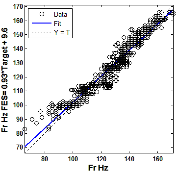
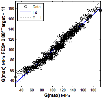
The rules were defined according to the MATLAB Fuzzy Logic Toolbox to construct the FES variables. Two built-in AND methods, min (minimum) and prod (product), and two built-in OR methods, max (maximum) and probor (probabilistic OR method),were used to evaluate the values of the resonant frequency and the maximum shear modulus. The best recall performances of the FES indicate that the system has an acceptable performance. The determination value (R 2 ) for the resonance frequency and the maximum shear modulus are shown in Fig. 2(a) and Fig. 2(b), respectively.
6. b) Generation of the Artificial Neural Networks (ANNs)
An artificial neural network is a soft computing technique that provides information processing by using the simulation of nerve cells and networks (Fahman, 1988). In this study, a supervised learning network using feed forward back propagation was performed. Alyuda NeuroIntelligence (ANI) software was used to design the structure of the neural network, and the network was compared with the other structures created by MATLAB. Various results were observed by selecting different layers and neurons. The dataset was formed by randomly separation method into training and validation. The Levenberg-Marquardt (LM) algorithm was used to train all the networks. LM was used because the algorithm is known as the optimum training algorithm and gives a virtual standard in nonlinear optimization. LM is a pseudo-second-order method, i.e., it does not only work with function evaluations and gradient information but also it estimates the Hessian matrix using the sum of the outer products of the gradients. LM quickly minimizes the error function and uses the Jacobian matrix instead of the Hessian matrix. The parameter, ?, is the Marquardt parameter, used in the calculation of the Hessian matrix (Hagan and Menhaj 1994).
H(n) = J T (n)J(n) + ?I(2)The weights and bias values are updated as follows:
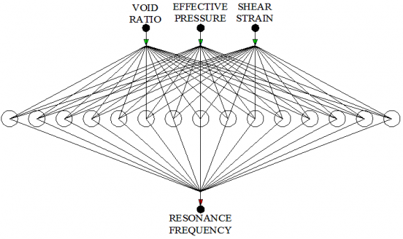
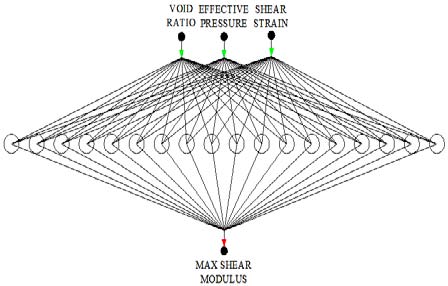
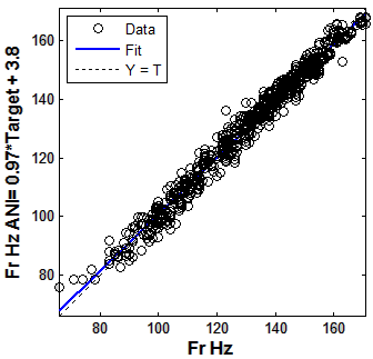
w(n + 1) = w(n) ? (H) ?1 J T (n)e(n)(3)The data for the input and output parameters are given in Table 4. An exhaustive search option in the ANI was used to choose the input variables. The optimal NN architecture was found as3-15-1 NN architecture for resonant frequencyand3-18-1 NN architecture for shear modulus. The NN architectures created by using Matlab NN are shown in Fig. 2. The same input variables were used and the linearity of the relationship between the parameters for the single-layer structure was found to be acceptable. The coefficients of determination value (R 2 ) (Y=T) are 0.9785 and 0.9787for the ANI predictions of resonance frequency and maximum shear modulus, respectively, which implies a significant value for R 2 and hence a good performance for the whole model. The results are presented in Fig. 3.
7. Resonant Frequency ANI Results
8. c) Generation of the Empirical Equation
The shear strain level is an important factor on the shear modulus. It is already known that the resonant column experiments are capable by achieving shear strain within an amplitude range of 10 -6 -10 -3 (Ishihara 2003).In any type of laboratory test, the shear modulus of cohesionless soils at low strain is measured under different effective confining stresses (?' 0 ) for various conditions presented by different void ratios (e). In the early works by Hardin and Richart(1972a-b), the effect of void ratio is found to be expressed by a function F(e): Thus, it is appropriate to divide the measured shear modulus (G max ) by the function F(e) and plot this ratio against the effective confining stress applied in the test (Kokusho 1987). The amplitude of the shear strain is obtained by converting the axial strain in the triaxial test through the following relationship:
F(e) =? a = (1 + ?)? a(5)A number of similar formulas are proposed for various sand types, as shown in Table 5; however, most of these formulas can be expressed in the general form of Eq.( 5).(Kokusho1987)For a sufficient small shear strain of ? a = 10 -5 , a typical formula is specified as Eq.( 6):
G 0 = AF(e)(? 0 ? ) n(6)G 0 = 8400
(2,17?e) 2 1+e (? 0 ? ) 0.5 (7) In this study, the experimental results were compared with the existing empirical relationships for the initial shear modulus obtained by performing various test devices for several types of sands at the shear strain of 10 -5 . All the results (0.001 ? ?% ? 0.04) of the empirical relationships were recomputed using the void ratio and the effective stress from the test results. The empirical relationship for the shear modulus given by Kokusho(1987)was found more appropriate for the values obtained from the test results in the range of the shear strain amplitude. The comparison between experimental results and literatureis shown in Fig. 4. The experimental test results were found to be in excellent agreement with the literature at a small shear strain amplitude. R 2 = 0.9111 (x = y) 0.001 ? ?% ? 0.04 R 2 = 0.9742 (x = y) 0.001 ? ?% ? 0.005 R 2 = 0.7452 (x = y) 0.005 < ?% ? 0.04 Fig. 4: Suitability of the experimental results and the Kokusho equation A new empirical relationship for the initial shear modulus was derived from the experimental studies at different shear strain levels by considering test data, the fuzzy expert system and the neural network results. Dynamic responses of soils can be determined atstrain levels between 10 -6 and 10 -2 by different test methods. But, decrease in shear modulus is observedfrom %0,005 strain levels to %0.0001 strain levels in the previous studies. Accuracy of the new equation was increased by considering boundary conditions at the shear strain ranges given by the ASTM standards for the resonant column test. Therefore, a new relationship to determine the initial shear modulus was divided into two parts given by Eq.( 8) and Eq.( 9).
In the range of 0.001 ? ?% ? 0.005, the equation is given below,
G0 = 8254 (2,17?e) 2 1+e (? 0 ? ) 0,49(8)In the range of 0.005 < ?% ? 0.04, the equation is given below,
G 0 = 7294 (2,17?e) 2 1+e (? 0 ? ) 0,49(9)The coefficients of determination value (R 2 ) (Y=T) are 0.9767 and 0.9362, respectively. Using these two equations for the prediction of the initial shear modulus, which implies a significant value for R 2 and indicates good performance for the whole model. The suitability of the derived empirical relationship according to the variation of the shear strain amplitude is shown in Fig. 5.
9. Conclusions
A series of RC tests was conducted on clean sand samples to create a new approach by using AI techniques for the prediction of the dynamic characteristics of soils. MATLAB software was used to perform data analysis and modeling. Test results were analyzed by considering saturation degree, effective stress and cyclic strain. First, two inference systems were performed to predict the maximum shear modulus and the database was created by using the experimental study. Compared with the test results, both inference system models were found to be quite suitable. Subsequently, new empirical relationships in the prediction of the dynamic characteristics of Toyoura sands were derived. New equation is divided in two groups by considering boundary conditions at the shear strain ranges given by the ASTM standards. Therefore, new formulation has a high level accuracy for determining the initial shear modulus of Toyoura sand samples. The equations showed acceptable results that were the analogous to those of the soft computing techniques. These results revealed that both methods can be used for practical purposes to solve complex real life problems. This study encourages further work to explore other inference systems for the estimation and generation of data from experimental studies.
V.
| Material | Toyoura Sand |
| D 50 (mm) | 0.26 |
| D 10 (mm) | 0.21 |
| C u | 1.33 |
| C c | 0.98 |
| G s | 2.653 |
| ? maks (Mg/m 3 ) | 1.34 |
| ? min (Mg/m 3 ) | 1.64 |
| e maks | 0.97 |
| e min | 0.597 |
| c (kPa) | 4 |
| ? | 39? |
| D 10 = |
| Year 2017 | ||||||||
| 32 | ||||||||
| ) Volume XVII Issue II Version I | ||||||||
| Global Journal of Researches in Engineering ( E | Max. | (e int ) 0.7959 | ? o '(kPa) 348.8 | %Dr 47.66 | H sample (mm) 135 | R sample (mm) 50 | %S r 99.98 | %? 0.04 |
| Min. | 06166 | 25.8 | 94.85 | 130 | 50 | 0 | 0.001 |
| Linguistic Rule | Abbreviations |
| Extremely High | VR7, EP6, G8, V6, FR7 |
| Very High | VR6, EP5, SS5, G7, V5, FR6 |
| High | VR5, EP4, SS4, G6, V4, FR5 |
| Medium High | G5 |
| Medium | VR4, SS3, FR4 |
| Medium Low | G4 |
| Low | VR3, EP3, SS2, G3, V3, FR3 |
| Very Low | VR2, EP2, SS1, G2, V2, FR2 |
| Extremely Low | VR1, EP1, G1, V1, FR1 |
| Total Sample:711 | e int | ? o '(kPa) | ?(%) | S r (%) | f r | G max (MPa) | V s (m/sn) |
| Column Type | Input | Input | Input | Input | Output | Output | Output |
| Format | Numerical | Numerical | Numerical | Numerical | Numerical | Numerical | Numerical |
| Scaling Range | [-1?1] | [-1?1] | [-1?1] | [-1?1] | [0?1] | [0?1] | [0?1] |
| Min | 0.6166 | 25.8 | 0.001 | 0 | 66 | 27.97 | 120.34 |
| Max | 0.7959 | 348.8 | 0.04 | 99.98 | 171 | 193.92 | 343.83 |
| Mean | 0.733718 | 150.83884 | 0.005447 | 60.76166 | 130.734177 | 112.976414 | 248.98495 |
| Std. Deviation | 0.046822 | 75.95824 | 0.006556 | 46.54837 | 21.815257 | 35.981497 | 45.01604 |
| References | A | F(e) | n | Soil Material | Test Method |
| Hardin-Richart (1963) | 7000 3300 | ? (2,17 ? e) 2 (1 + e) (2,97 ? e) 2 (1 + e) ? | 0,5 0,5 | Round Grained Crashed Quartz Ottowa Sand Angular Grained | Resonant Column |
| Shibata-Soelarno (1975) | 42000 | (0,67 ? e) (1 + e) ? | 0,5 | Three types of clean sand | Ultrasonic Pulse |
| Iwasaki et.al. (1978) | 9000 | (2,17 ? e) 2 (1 + e) ? | 0,38 | Eleven types of clean sand | Resonant Column |
| Kokusho (1980) | 8400 | (2,17 ? e) 2 (1 + e) ? | 0,5 | Toyoura Sand | Cyclic Triaxial |
| Yu-Richart (1984) | 7000 | (2,17 ? e) 2 (1 + e) ? | 0,5 | Three types of clean sand | Resonant Column |
| ?? ?? :kPa; ð??"ð??" ?? ? :kPa; e: void ratio | |||||