1. I. Introduction
he focus of this research is to address the challenges of electrical power distribution systems in Nigeria. The relationship between the input and output of a single-input-single-output electrical power distribution system although fairly known, but it is least understood. A major reason for this is that electrical power distribution system transfer function which serves as a guide for measuring and monitoring electrical power distribution output is often never determined and factored into the distribution control system. The decision problem is which analytical technique to adopt to clarify the nature of the relationship. In this study, the transfer function model is employed. Transfer function modeling is an integral part of control and process monitoring which is used to determine the causal relationship between input and output of a process. Efforts at relating the input to output of a system statistically started with regression analysis (Lai, 1979). Hence, regression analysis formed the basis of the traditional statistical method of modeling the relationship between the input and output to systems. Regression analysis has many deficiencies, for example; regression analysis is inappropriate in situations where the output lags the input when there is a significant amount of noise in the system regression analysis cannot accommodate noise in the filter (Box and Jenkins, 1994).
In 1970, Box and Jenkins introduced an improved statistical method of modeling the relationship between the input and output to a system. This method was named Box-Jenkins transfer function modeling methodology (Lai, 1979). Box et al did a very significant work in transfer function modeling by introducing ARIMA and noise models into transfer function modeling. This significantly improved the efficiency and reliability of transfer function models. In addition to this, transfer function model forecasts usually have smaller forecasting errors than the forecasts based on univariate models which are based on the output, and gives good forecasts of the future output from a process which is very significant. Since the introduction of transfer function modeling in 1970, efforts have been made by various researchers to improve and extend its application in various fields of life. For example Lai (1979) This work is therefore conceived to explore transfer function modeling as a possible monitoring and control tool for improving the operational efficiency of an electrical power distribution system. The hub of our investigation is Shell Forcados Terminal located Southwest of Warri, Delta State Nigeria.
2. II. The General Transfer Function Modelling Procedure
A discrete transfer function model applicable to a distribution process has been developed by Box et al. We shall assume the model as stated in equation (3.1) as follows:
?? ??=?? ?1 (??)ð??"ð??"(??)?? ????? + ?? ?? (3.1)The noise term, ?? ?? , is represented by an ARIMA (p,d,q) process such that:
?? ??=?? ?1 (??)??(??)?? ?? (3.2)Here ?? ?? is the white noise. Substituting equation (3.2) into (3.1), gives
?? ??=?? ?1 (??)ð??"ð??"(??)?? ????? + ?? ?1 (??)??(??)?? ?? (3.3)3. III. Methodology
The basic model used in this research is the transfer function modeling. The transfer function modeling procedure consists of the following steps: 3), a plot of the 4-month inputoutput data was done using SPSS software. After the plot, the data was investigated for stationarity, using the plots of the autocorrelation functions (ACF) and Pearson's autocorrelation functions (PACF). The input and output series derived from the plots were found not to be stationary, hence differencing was used to achieve stationarity. Stochastic regularity was achieved after the second differencing. Following the achievement of stationarity of the input ?? ?? and output ?? ?? , univariate model was individually fitted to ?? ?? and ?? ?? in order to respectively estimate pre-whitened input and output series namely ?? ?? and ?? ?? . Calculation of the cross correlation function was used to identify r, s and b parameters of the transfer function model.
Furthermore, the transfer function was estimated using ?? ?? and ?? ?? . The residual of the transfer function was used to identify the noise term ?? ?? of the transfer function model. Finally, the model adequacy check and optimization was done using genetic algorithm.
As transfer function model parameters are continuous variables, the genetic algorithm method was the continuous version. The model parameters are: b, ?, ?, ? and ? as shown in equation (3.3).
4. IV. Results
Transfer Function Modelling: The data gotten from transformer (TR-102) at switchgears SG-101(Input) and SG-102 (Output) at Shell Forcados Power Terminal was analyzed in line with the theory and procedure developed and described earlier in the methodology.
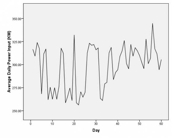
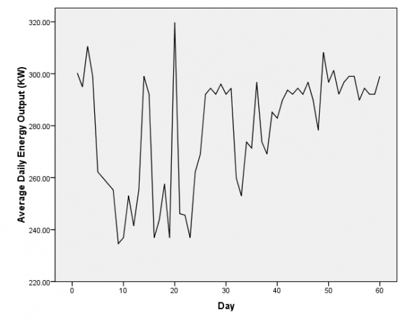
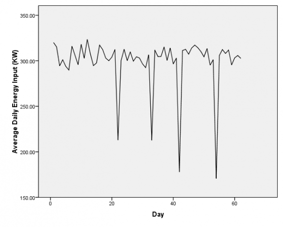
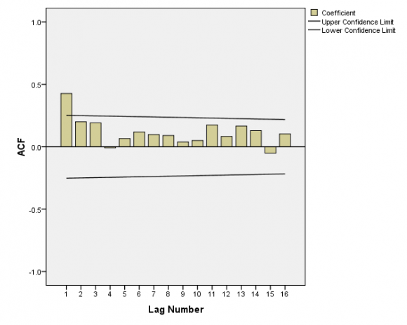
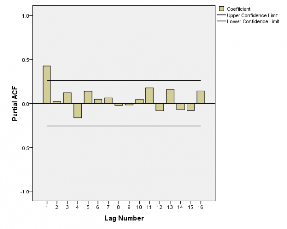
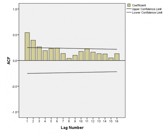
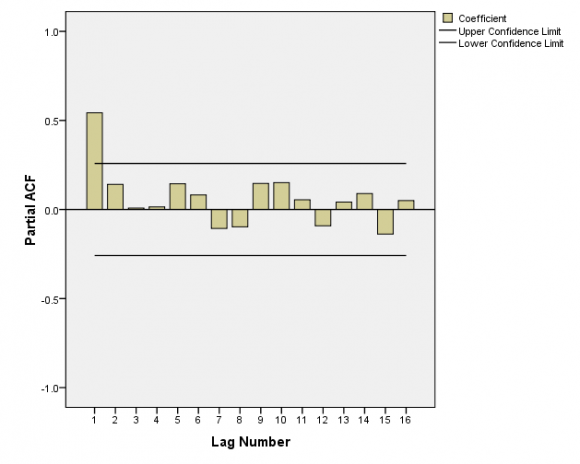
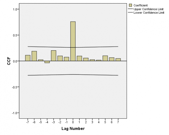
The abscissas of Figures 1 to 4 are in days-ofthe month (30). The distribution station is supplied with 33kv from the national grid and it is stepped down to 11kv for distribution to consumers. The power input depends on availability of power in the national grid which is fed by the generation stations. Thus as shown in Figures 1 and 3, the power supply does not follow any particular pattern. The output power depends on demand and the conditions of the distribution facilities. Hence, the output time series of Figures 2 and 4 follow the pattern described in the foregoing. The input series upon analysis was found to be stationarity, hence differencing was not used. Examination of the ACF and PACF in Figures 4 and 5 are indicative that auto regression one (AR (1)) model is the appropriate model to use. The formula for AR (1) models [2, 14 and 15] is given by equation ( 4): The output series upon analysis was found to be stationarity, hence differencing was not used. Examination of the ACF and PACF in Figures 5 and 6 are indicative that auto regression one (AR (1)) model is the appropriate model to use. The CCF between ? t and ? t is shown in Figure 5.3.2. It has one significant CCF at lag zero (0).Hence, according to [14], the parameters r, s and b of the transfer function that supports such CCF pattern are 0, 0 and 0 respectively. In view of this fact, the CCF supports the following transfer function model:
0 t N t x t y + = ?Based on Ljung-Box statistics shown in Table 5.3 and analysis of the residuals, the transfer function was found to have white noise residuals, hence we disregarded the noise term t N , to obtain equation (22). The lag of 0 in the transfer function model shows that the average gas flow in the month is used for generation the same month. The model has intuitive and theoretical appeal. The model fit and statistics are good as shown for month 1-2 in Tables 1 and 2 respectively. The lag of 0 in the transfer function model shows that the average gas flow in the month is used for generation the same month. The model has intuitive and theoretical appeal. The model fit and statistics are good as shown for the month 3-4 in Tables 2 and 3 respectively.


![Figure 8 : PACF of the output series The formula for AR (1) models [2, 14 and 15] is given by equation (12):](https://engineeringresearch.org/index.php/GJRE/article/download/1532/version/101409/5-Modeling-of-the-Transfer_html/30173/image-7.png)
| it Statistic | Value |
| Stationary R-squared | .712 |
| R-squared | .712 |
| MSE | 12.362 |
| MAPE | 3.407 |
| MaxAPE | 12.212 |
| MAE | 9.300 |
| MaxAE | 30.309 |
| Normalized BIC | 5.234 |
| Model Fit | ||||||
| Model | Number of Predictors | statistics Stationary R-squared | Statistics | Ljung-Box Q(18) DF | Sig. | Number of Outliers |
| Transfer Function Model | 1 | .712 | 9.592 | 17 | .920 | 0 |
| For month 1-2 operations of the Power Station we | ||||||
| obtained: | ||||||
| Fit Statistic | Value |
| Stationary R-squared | .587 |
| R-squared | .067 |
| RMSE | 31.836 |
| MAPE | 7.766 |
| MaxAPE | 80.056 |
| MAE | 18.033 |
| MaxAE | 131.997 |
| Normalized BIC | 7.123 |
| Months | Total Energy Output | Coefficient of | |
| (MWH) | Performance | ||
| ? | 0 | ||
| 1-2 | 401.32 | 0.670 | |
| 3-4 | 432.73 | 1.065 | |