1. I. Introduction
major problem that faces highway and transportation agencies is that the funds they receive are usually insufficient to adequately repair and rehabilitate every roadway section that deteriorates. The problem is further complicated in that roads may be in poor condition but is still unable; making it easy to defer repair projects until conditions becomes unacceptable. Roadway deterioration usually is not the result of poor design and construction practices but is caused by the inevitable wear and tear that occurs over years. The gradual deterioration of a pavement occurs due to many factors including variations in climate, drainage, soil conditions, and truck traffic. Just as a piece of cloth eventually tears asunder if a small hole is not immediately repaired, so will a roadway unravel if its surface is allowed to deteriorate. Lack of funds often limits timely repair and rehabilitation of transportation facilities, causing a greater problem with more serious pavement defects and higher costs (Garber and Hole 2009).
In order to carry out the maintenance in as costeffective manner as possible, a logical coherent procedure must be adopted in order to select the most effective form that the maintenance should take, together with the optimum time at which this work should be undertaken. Minor maintenance may be sufficient to maintain the required standard of service for the motorist (Rogers 2003).
The AHP is a general theory of measurement. It is used to derive relative priorities on absolute scales (invariant under the identity transformation) from both discrete and continuous paired comparisons in multilevel hierarchic structures. These comparisons may be taken from actual measurements or from a fundamental scale that reflects the relative strength of preferences and feelings. The AHP has a special concern with departure from consistency and the measurement of this departure, and with dependence within and between the groups of elements of its structure. It has found its widest applications in multicriteria decision making (Saaty and Elexander 1989) in planning and resource allocation (Saaty 2005), and in conflict resolution. In its general form, the AHP is a nonlinear framework for carrying out both deductive and inductive thinking without use of the syllogism. This is made possible by taking several factors into consideration simultaneously, allowing for dependence and for feedback, and making numerical tradeoffs to arrive at a synthesis or conclusion (Saaty and Vargas 2006).
The foundation of the Analytic Hierarchy Process (AHP) is a set of axioms that carefully delimits the scope of the problem environment (Saaty 1996). It is based on the well-defined mathematical structure of consistent matrices and their associated righteigenvector's ability to generate true or approximate A Global Journal of Researches in Engineering ( ) Volume XVI Issue V Version I weights. The AHP methodology compares criteria, or alternatives with respect to a criterion, in a natural, pairwise mode. To do so, the AHP uses a fundamental scale of absolute numbers that has been proven in practice and validated by physical and decision problem experiments. The fundamental scale has been shown to be a scale that captures individual preferences with respect to quantitative and qualitative attributes just as well or better than other scales (Saaty 1980). It converts individual preferences into ratio scale weights that can be combined into a linear additive weight w (a) for each alternative.
The resultant w (a) can be used to compare and rank the alternatives and, hence, assist the decision maker in making a choice. Given that the three basic steps are reasonable descriptors of how an individual comes naturally to resolving a multicriteria decision problem, then the AHP can be considered to be both a descriptive and prescriptive model of decision making. The AHP is perhaps, the most widely used decision making approach in the world today. Its validity is based on the many hundreds (now thousands) of actual applications in which the AHP results were accepted and used by the cognizant decision makers (DMs) (Vahidnia et.al. 2008).
2. a) Decision Making of Multiple Criteria Sealing
The analytic hierarchy process (AHP) is a basic approach to decision making. This multiple criteria scaling method was founded by Saaty (1977). It is designed to cope with both the rational and the intuitive to select the best from a number of alternatives evaluated with respect to several criteria. In this process, the decision maker carries out simple pairwise comparison judgments. These are used to develop overall priorities for ranking the alternatives. The AHP both allows for inconsistency in the judgments and provides a means to improve consistency. The procedure starts with development of alternative options, specification of values and criteria, then, it follows the evaluation and recommendation of an option (Farkas 2010).
3. b) Philosophy of AHP
The AHP is a general theory of measurement. It is used to derive the most advanced scales of measurement (called ratio scales) from both discrete and continuous paired comparisons in multilevel hierarchic structures. These comparisons may be taken from actual physical measurements or from subjective estimates that reflect the relative strength of preferences of the experts (Farkas 2010).
The AHP is a method that can be used to establish measures in both the physical and human domains. The AHP has special concern with departure from consistency and the measurement of this departure, and dependence within and between the groups of elements of its structure. This is made possible by taking several factors into consideration simultaneously, allowing for dependence and for feedback, and making numerical tradeoffs to arrive at a synthesis or conclusion (Saaty 1996).
In using the AHP to model a problem, one needs a hierarchic structure to represent that problem, as well as pairwise comparisons to establish relations within the structure. In the discrete case, comparisons lead to dominance matrices and in the continuous case to kernels of Fredholm operators, from which ratio scales are derived in the form of principal eigenvectors, or eigen functions, as the case may be. These matrices, or kernels, are positive and reciprocal. In a real world application of the AHP the required number of such matrices is equal to the number of the weighting factors. In addition, regarding that the number of the group members is 5-15, there is a need for aggregation what is called the process of synthesizing group judgments. By synthesizing the particular priorities with the average weighting factors of the attributes the ultimate output is yielded in the form of a weighted priority ranking indicating the overall preference scores for each of the alternatives under study (Saaty and Vargas 2006).
The AHP procedure involves six essential steps (Vahidnia et.al. 2008):
4. Define the unstructured problem
In this step the unstructured problem and their characters should be recognized and the objectives and outcomes stated clearly.
5. Developing the AHP hierarchy
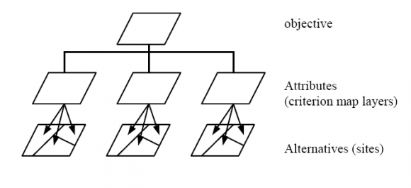
The first step in the AHP procedure is to decompose the decision problem into a hierarchy that consists of the most important elements of the decision problem. In this step the complex problem is decomposed into a hierarchical structure with decision elements (objective, attributes i.e. criterion map layer and alternatives).
6. Pairwise Comparison
For each element of the hierarchy structure all the associated elements in low hierarchy are compared in pairwise comparison matrices as follows:
A = ? ? ? ? ? ? 1 ?? 1 ?? 2 ? ?? 1 ?? ?? ?? 2 ?? 1 1 ? ?? 2 ?? ?? ? ? ? ? ?? ?? ?? 1 ?? ?? ?? 2 ? 1 ? ? ? ? ? ?(1)where A = comparison pairwise matrix, w 1 = weight of element 1, w 2 = weight of element 2, w n = weight of element n.
In order to determine the relative preferences for two elements of the hierarchy in matrix A, an underlying semantically scale is employs with values from 1 to 9 to rate.
7. Estimating the relative weights
Some methods like eigenvalue method are used to calculate the relative weights of elements in each pairwise comparison matrix. The relative weights (W) of matrix A is obtained from following equation:
(A -? max I ) × W =0 (2)where ? max = the biggest eigenvalue of matrix A, I= unit matrix. From the standpoint of engineering applications, eigenvalue problems are among the most important problems in connection with matrices.
Let A = [a jk ] be a given n×n matrix and consider the vector equation:
Ax = ?x (3)Here, x is an unknown vector and ? an unknown scalar. Clearly, the zero vector x=0 is a solution of equation ( 3) for any value of ?. This is of no practical interest. A value of ? for which (4.3) has a solution x?0 is called an eigenvalue or characteristic value (or latent root) of matrix A. The corresponding solutions x?0 of equation ( 3) are called eigenvectors or characteristic vectors of A corresponding to that eigenvalue ?. The set of Eigenvalues is called the spectrum of A. The largest of the absolute values of the eigenvalues of A is called the spectral radius of A.
8. Checking the consistency
In this step the consistency property of matrices is checked to ensure that the judgments of decision makers are consistent. For this end some pre-parameter is needed. Consistency Index (CI) is calculated as (Vahidnia et.al. 2008):
CI = ?? ?????? ? ?? ???1 (4)The consistency index of a randomly generated reciprocal matrix shall be called to the random index (RI), with reciprocals forced. An average RI for the matrices of order 1-15 was generated by using a sample size of 100.
Table (1) shows random indexes of the matrices of order 1-15 (Coyle 2004). The last ratio that has to be calculated is CR (Consistency Ratio). Generally, if CR is less than 0.1, the judgments are consistent, so the derived weights can be used. The formulation of CR is: Figure (2) developed from table 2 to determine the random index (RI) for all sizes of matrices (n) and create the following equation from that graph by using least square polynomial method: y= a 0 + a 1 x+ a 2 x 2 + a 3 x 3 [R 2 =0.9766] (6) where a 0 =0.6304, a 1 =0.5222, a 2 =0.0430, a 3 =0.0012 6. Obtaining the overall rating In last step the relative weights of decision elements are aggregated to obtain an overall rating for the alternatives as follows (Vahidnia et.al. 2008):
CR = ???? ???? (5)W i S = ? ?? ???? ?? ?? ??? ?? ?1 ?? ?? ?? i = 1,?,n(7)where W i S = total weight of site i, w ij S = weight of alternative (site) i associated to attribute (map layer) j, w j a = weight of attribute j, m = number of attribute, n= number of site.
9. c) Modeling the Decision Making with AHP for Treatment Selection of pavement
The first step in the AHP procedure is to decompose the decision problem into a hierarchy that consists of the most important elements of the decision problem. In developing a hierarchy identified the objective, factors and alternatives. The hierarchy model of a decision problem is the objective of the decision at the top level and then descends downwards lower level of decision factors until the level of attributes is reached. Each level is linked to the next higher level.
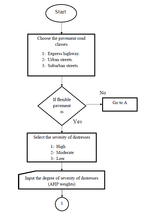
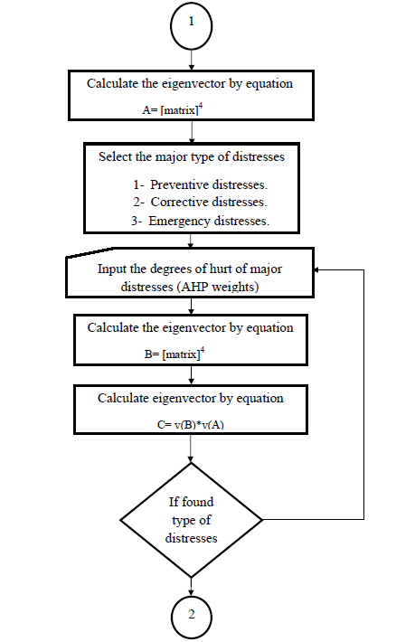
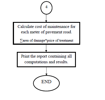
Decision making with AHP for treatment selection of pavement is modeled as a program by using MATLAB 2008a. Figure (3) illustrates the flowchart of the developed program for modeling AHP as the basic form of a hierarchical model of making decision, where the objective to identify suitability for choosing the type of maintenance activity. This can be achieved in the following nine steps:
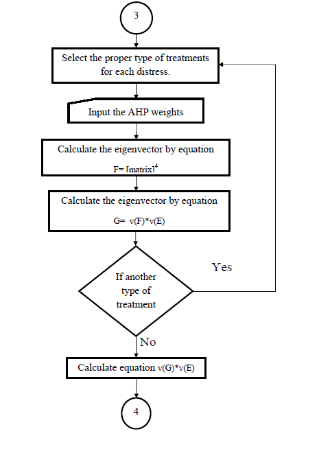
1. Ranking the highway road (classes of road): express highway, urban streets and suburban streets. 2. Defining the type of pavement, flexible pavement or rigid pavement. 3. Defining the severity of distresses, low, moderate and high then input the degree of severity of distresses as weights of important of intensity (AHP process), and solve the compared matrix by eigenvector. 4. Selecting the major types of distresses, preventive distress, corrective and emergency distress, then input the degree of hurt of major distress as weights of important of intensity (AHP process), and calculated the compared matrix by eigenvector. 5. Multiplying the eigenvectors calculated from step 4 by eigenvector calculated from step3. 6. Selecting the type of minor distress: for flexible pavement; cracking, raveling rutting, distortion potholes and excess asphalt. For rigid; joint distress, faulting, pattern cracking, surface distress and slab cracking. Input the degree of hurt of minor distress as weights of important of intensity (AHP process), then calculate the compared matrix. 7. Multiplying the eigenvectors result from step 6 by eigenvector result from step 5. 8. Selecting the proper type of treatments for each distress. Input the weights of important of intensity (AHP process) for the treatments then calculate the compared matrix. 9. Multiplying the eigenvectors result from step 8 by eigenvector result from step 7, then select the treatment that its number equal to ? max .
10. d) Development of the Comparison Matrix
In this stage the researchers conducted many personal interviews with senior engineers who have an experience in road maintenance projects. About 6 senior engineers were selected to conduct the interviews. Every engineer of those experts gave pairwise comparison matrices as weights of AHP process.
11. II. Case Study
The case study is a local road of University of Baghdad, which is begin from gate of University of Baghdad returned as a ring to the gate with length 2.38 Km and width 7 m with 2-lane and one way, as it is clear in figure (4). Table 2 shows the distresses types of this case study (University of Baghdad street).
12. the pairwise comparison matrix
There are 12 pairwise comparison matrices in all: One for the criteria with respect to the goal, which is shown here in Table 4, two for the subcriteria, the first of which for the subcriteria under high distresses: preventive, corrective and emergency, that is given in Table 5 and one for the subcriteria under moderate distresses that is given in Table 6.
Then, there are nine comparison Saaty matrices for the four alternatives with respect to all the 'covering criteria', the lowest level criteria or subcriteria connected to the alternatives. The 9 covering criteria are: corrective distresses, emergency distresses, and edge cracking treatment, block cracking treatment, transverse cracking treatment, longitudinal cracking treatment, and alligator cracking treatment, potholes distress treatment, and raveling distress treatment.
The comparisons matrices of this case are calculates as then shown in the four tables below (from table 3 to table 6). For subcriteria (distresses of pavement), a comparison matrix shown in table 7 with respect to corrective maintenance, the eigenvector of relative importance for E, B, T, L, A, P and R is (0.1065, 0.08, 0.1489, 0.2142, 0.3182, 0.0818, 0.0504), where E, B, T, L, A, P and R is abbreviation for edge cracks, block cracks, transverse cracks, longitudinal cracks, alligator cracks, potholes distress and raveling distress respectively. Table 11 shows results of priorities of judgments for six experts and average of their judgments. Where 1, 2, 3, 4, 5 and 6 represent expression of six experts and 7 the average of their judgments. The eigenvector of the relative importance or value of distresses treatments is varying in values according the judgments of experts. For expert number 1, TC is the most valuable and MS, CP and HP are less significant. For expert number 2, F is the most valuable and MS, CP and HP are less significant. For expert number 3, SC is the most valuable and MS, CP and HP are less significant. For experts numbers 4 and 5, F is the most valuable and MS, CP and HP are less significant. For expert number 6, TC is the most valuable and MS, CP and HP are less significant. From the average of judgments of experts, TH is the most valuable and MS, CP and HP are less significant.
13. III. Conclusions
The conclusions drawn from this work can be summarized as follows: 1. The analytic hierarchy process (AHP) is an excellent method, which has been applied in this study for estimating the relative weighs of different factors that considered in spatial analysis process to the case of selecting a proper treatment for pavement. It provides a convenient approach for solving complex MCDM problems in engineering. The main advantage of the AHP is its ability to rank choices in the order of their effectiveness in meeting conflicting objectives.
14. The developed program AHPM (Analytic Hierarchy
Process Model) is written by using MATLAB2008a. It can determine the best treatment for damages of pavements. The AHPM contains nine steps for choosing the type of maintenance activity of asphalt and rigid pavement. Those steps include the inputs of elements (criteria, sub-criteria and alternatives) of asphalt pavement and rigid pavement as weighs of important of intensity. 3. In this study, comparisons matrices were developed as weighs of AHP process according to judgments of experts who have an experience in road maintenance projects. 4. The (AHPM) software was applied to a case study, which was a main road of University of Baghdad.
The result was yielding an asphalt thin hot mix overlay as the required maintenance activity.
| N 1 2 | 3 | 4 | 5 | 6 | 7 | 8 | 9 | 10 | 11 | 12 | 13 | 14 | 15 | |
| RI 0 | 0 | 0.58 | 0.9 | 1.12 | 1.24 | 1.32 | 1.41 | 1.45 | 1.49 | 1.51 | 1.48 | 1.56 | 1.57 | 1.59 |
| Year 2016 | |||
| 30 | |||
| Distress type | Severity level | Extent level | |
| 1 | Edge cracks | Moderate | High |
| 2 | Block cracks | High | Very high |
| 3 | Transverse cracks | Very high | High |
| 4 | Longitudinal cracks Alligator | Moderate | Low |
| 5 | cracks | High | Moderate |
| 6 | Potholes | High | Moderate |
| 7 | Raveling | High | Moderate |
| Low | Moderate | High | 4 th root of product of values | Eigenvector (Priorities) | |
| Low | 1 | 1/3 | 1/5 | 48.2522 | 0.1007 |
| Moderate | 3 | 1 | 1/4 | 108.0709 | 0.2256 |
| High | 5 | 4 | 1 | 322.6167 | 0.6736 |
| Total | 478.9398 | ?1.000 | |||
| ? max = 3.086 , CI= 0.043, | RI= 0.58, | CR= 0.074?0.1 o.k | |||
| Year 2016 | |||||
| 31 | |||||
| ( ) Volume XVI Issue V Version I | |||||
| of Researches in Engineering | |||||
| Global Journal | |||||
| Preventive | Corrective | Emergency | 4 th root of product of values | Eigenvector (Priorities) | |
| Preventive | 1 | 1/3 | 1/7 | 45.3283 | 0.0810 |
| Corrective | 3 | 1 | 1/5 | 105.4457 | 0.1885 |
| Emergency | 7 | 5 | 1 | 408.7524 | 0.7305 |
| Total | 559.5264 | 1.00 |
| ? max = 3.104 , CI= 0.052, | RI= 0.58, | CR= 0.09 ?0.1 o.k |
| Moderate | High | Eigenvector | |
| (0.2256) | (0.6736) | (Priorities) | |
| Preventive | 0.0810 | 0.0705 | 0.0658 |
| Corrective | 0.1885 | 0.1532 | 0.1457 |
| Emergency | 0.7305 | 0.7705 | 0.6838 |
| ? max = 7.567, CI= 0.095, | RI= 1.32 , | CR= 0.072 ?0.1 o.k |
| Table 8 shows the comparison matrix for | eigenvector of relative importance for A, P and R is | |
| distresses with respect to emergency maintenance. The | (0.5396, 0.297, 0.1634) respectively. | |
| ? max = 3.009 , CI= 0.005, | RI= 0.58 , | CR= 0.008 ?0.1 o.k |
| Corrective | Emergency | Eigenvector | ||
| (0.1457) | (0.6838) | (Priorities) | ||
| E | 0.1065 | 0 | 0.0155 | |
| B | 0.0800 | 0 | 0.0117 | |
| T | 0.1489 | 0 | 0.0217 | |
| L | 0.2142 | 0 | 0.0312 | |
| A | 0.3182 | 0.5396 | 0.4153 | |
| P | 0.0818 | 0.297 | 0.2150 | |
| R | 0.0504 | 0.1634 | 0.1191 | |
| Finally the final overall priorities of treatments of | (0.0286, 0.0162, 0.0292, 0.0494, 0.0523, 0.0753, 0, | |||
| distresses calculated by multiplying the eigenvectors of | 0.0194, 0, 0, 0.1609, 0.2063, 0.0771, 0.0603 and 0.0541) | |||
| treatments of distresses by the eigenvector of types of | respectively. Thus, TH is the most valuable and MS, CP | |||
| distresses that shown in table 10. From table 10 the | and HP are less significant. | |||
| eigenvector of the relative importance or value of D, C, | ||||
| F, SC, SL, CH, MS, M, CP, HP, TC, TH, PA, O and RE is | ||||
| E | B | T | L | A | P | R | Overall | |
| (0.0476) | (0.2252) | (0.2962) | (0.1473) | (0.1249) | (0.0848) | (0.074) | Priorities | |
| D | 0.0564 | 0.0627 | 0.0573 | 0.0801 | 0.0201 | 0.0392 | 0.0546 | 0.0286 |
| C | 0.1310 | 0.0878 | 0.0682 | 0.3725 | 0 | 0 | 0 | 0.0162 |
| F | 0 | 0.0993 | 0.0963 | 0 | 0.0447 | 0 | 0.0619 | 0.0292 |
| SC | 0 | 0.0712 | 0.0810 | 0.2530 | 0.0617 | 0 | 0.1114 | 0.0494 |
| SL | 0 | 0.1538 | 0.1373 | 0 | 0.0921 | 0 | 0.0780 | 0.0523 |
| CH | 0 | 0.1179 | 0.1633 | 0.1799 | 0.1129 | 0 | 0.1503 | 0.0753 |
| MS | 0 | 0 | 0 | 0 | 0 | 0 | 0 | 0 |
| M | 0 | 0 | 0.1203 | 0 | 0 | 0.0780 | 0 | 0.0194 |
| CP | 0 | 0 | 0 | 0 | 0 | 0 | 0 | 0 |
| HP | 0 | 0 | 0 | 0 | 0 | 0 | 0 | 0 |
| TC | 0.2388 | 0.1738 | 0 | 0 | 0.2077 | 0.2154 | 0.1895 | 0.1609 |
| TH | 0.5737 | 0.2336 | 0 | 0 | 0.2980 | 0.1354 | 0.3512 | 0.2063 |
| PA | 0 | 0 | 0.2763 | 0.1145 | 0.1627 | 0 | 0 | 0.0771 |
| O | 0 | 0 | 0 | 0 | 0 | 0.2805 | 0 | 0.0603 |
| RE | 0 | 0 | 0 | 0 | 0 | 0.2515 | 0 | 0.0541 |
| ( ) Volume XVI Issue V Version I | |||||||
| of Researches in Engineering | |||||||
| Global Journal | |||||||
| Experienced | |||||||
| Overall | 1 | 2 | 3 | 4 | 5 | 6 | 7 Average |
| priorities | |||||||
| D | 0.0361 | 0.0280 | 0.0404 | 0.0296 | 0.0529 | 0.0456 | 0.0286 |
| C | 0.0080 | 0.0118 | 0.0186 | 0.0231 | 0.0337 | 0.0067 | 0.0162 |
| F | 0.0484 | 0.1304 | 0.1368 | 0.1822 | 0.1567 | 0.0449 | 0.0292 |
| SC | 0.0552 | 0.1138 | 0.1422 | 0.1383 | 0.1538 | 0.0353 | 0.0494 |