1. Introduction
he Tranposrt phenomena in geomechanics is a complex problem and cover a wide range of application. Problem as the contamination of land in many countries or recovery of oil in reservoir e.t.c, are dominated from the uncertainty and spatial variability of the properties of soil materials. Various forms of uncertainties arise which depend on the nature of geological formation, the extent of site investigation, the type and the accuracy of design calculations etc. In recent years there has been considerable interest amongst engineers and researchers in the issues related to quantification of uncertainty as it affects safety, design as well as the cost of projects.
Zhang, P. and Hu, L. (2014) presented in their study, a generalized model of preferential flow paths based on a dual-domain model which reflects contaminant transport and the dynamic transfer between two domains, and quantitatively analyzes the difference between advection-dispersion model (ADM) and dual-domain mass transfer model (DDM) in pore scale. Basic idea of this paper was the complexity of contaminant transport through highly heterogeneous soil on predicting pollution of the soil and groundwater system. Mousavi et all (2013) presented the development and the application of a numerical model for simulation of advective and diffusive-dispersive contaminant transport using a stochastic finite-element approach. Employing the stochastic finite-element method proposed in this study, the response variability was reproduced with a high accuracy. Johnson et all (2010) introduced an approach which has been incorporated into a spreadsheet model which uses a one-dimensional solution to the advection dispersion equation, which readily lends itself to Monte Carlo applications. The scope of this work was the definition of contaminant source release of contaminant mass transport simulation in the saturated zone as many sites the release history is unknown. Nadim et all (2004) proposed a three-dimensional stochastic model for the generation and transport of LFG in order to quantify the uncertainties. Using Monte Carlo simulations, multiple realizations of key input parameters was generated. For each realization, LFG transport was simulated and then used to evaluate probabilistically the rates and efficiency of energy recovery. Wörman, A. and Xu, S. (2001) developed a new modeling framework for internal erosion in heterogeneous stratified soils by combining existing methods used to study sediment transport in canals, filtration phenomena, and stochastic processes. The framework was used to study the erosion process in sediments caused by a flow of water through a covering filter layer that deviates from geometrical filter rules. By the use of spectral analysis and Laplace transforms, mean value solutions to the transport rate and the variance about the mean was derived for a transport constraint at the upstream boundary and a constant initial transport.
In this paper we present a general SFEM for transport phenomena in geomechanics using the method of Generalized Polynomial Chaos (GPC). In the first part of the paper a new algorithm based on RFEM using the Circulant Embedding method (Lord et all 2014) is presented in order to generate the random fields. In the second part, development of SFEM based on the Karhunen-Loeve Expansion for stochastic process discretisation and GPC is described. Finally in the last part of the paper, the problem of contamination of soil due to a surface source is solved by the two methods and the results are compared. and characterized by specific distribution. The Gaussian distribution is the default distribution in most application of probabilistic engineering mechanics. In our case the Gaussian distribution is inappropriate because of coefficients' nature. None of them cannot take negative value. Thus in order to cover all the values of them greater than zero a long normal distribution is adopted.
The expected value of a quantity of the problem is given by the following norm:
??? ?? 2 ???,?? 2 (??)? = ? ? |?| 2 (??, ð??"ð??")??????? ?? ?? = ð?"¼ð?"¼???? ?? 2 (D) ?(2)In essence the solution of the problem is a function of the form ?? ?? ? ?? × ?? ? ? for every fixed t, i.e. a random field and is not a deterministic function.
II.
2. Random Finite Element
The most common way to solve this problem is to create a random field of the soil properties which is mapped to a grid of finite element and then for different every time realization of the fields {?? ???? ( ?? , ??) : ? ?? × ??} {??( ?? , ??) : ? ?? × ??} and the source or sink {??( ?? , ??) : ? ?? × ??} to solve an ordinary boundary value problem using the Monte Carlo method. Assuming the same randomness for all leads to computational efficiency and is not far from the reality.
In the current work the random field is generated by the Circulant Embedding method (Lord et all 2014) using the Fast Fourier Algorithm resulting, as will be shown in the following sections, an exact simulation of stochastic processes.
Following the random field generation the displacement field ?? ?? (??) for each realization is taken place. At the end of all running the statistical moment based on the Monte Carlo method is calculated. The problem for each realization of ??? ???? ( ?? , ??) : ? ?? × ??? and the source or sink {??( ?? , ??) : ? ?? × ??} is:
? ???? ?? (??,And the expected values at the end:
ð?"¼ð?"¼(??(??)) = 1 ?? ? ?? ?? (??) ?? ??=1(6)And the variance
??????(??(??)) = 1 ?? ? 1 ?(?? ?? (??) ? ð?"¼ð?"¼(??(??)) 2 ?? ??=1(7)III.
3. Random Field Generation
The Circulant Embedding method (Lord et all 2014) is a technique used for the generation of realizations of Gaussian stochastic processes. This technique has two main advantages among others. The first is that the statistical properties of the generated process are exactly the same process that we aim. The second advantage arises from the Fast Fourier Transform Algorithm which significantly reduces the computational cost. This method seems to have initially been studied in problems of one dimension by Davies & Harte (1987) and more systematically by Dembo et al. (1989), Dietrich & Newsam (1993, 1997), Gneiting (2000), Stein (2001), Craigmile (2003), andPercival (2006). Extension of the method to a multi-parameter problems studied by Wood (1999), Helgasonetal (2011) whereas in random fields by Dietrich & Newsam (1993), Wood & Chan (1994, 1997), Stein (2002Stein ( , 2012)), Gneiting et al. (2006). Considerable work was recently featured by Lord et all (2014) whose principles are followed in this work. According to the method, in the case where the samples are uniformly distributed in space in a twodimensional problem, then the covariance matrix C is Toeplitz (Appendix A) and has as elements Toeplitz blocks (block Toeplitz with Toeplitz blocks (BTTB)). The covariance matrix can be described by the Fast Fourier Algorithm:
?? = ?????? ??(8)Where:
?? ??=?? 1 ?? 2 ×?? 1 ?? 2 = ?? 1 ??? 2 (9)The F 1 , F 2 are the Fourier matrices with dimension of n 1 × n 1 and n 1 × n 2 respectively and the diagonal matrix D includes the eigenvalues of the covariance matrix. For the application of the method the covariance matrix has to be circulant and for that reason using the BTTB matrix invokes a new circulant ((Appendix A)) matrix is created with ?? 2 blocks of circulant matrices ?? 1 × ?? 1 which is represented uniquely by the reduced matrix ?? ð??"ð??"ð??"ð??"ð??"ð??" = [?? 0 , ? , ?? n 2 ?1 ]. The latter can be replaced uniquely by the vector ?? ð??"ð??"ð??"ð??"ð??"ð??" ? ? n 1 n 2 .
Following the process described and provided that the covariance matrix has non-negative and real eigenvalues we get: Where:
?? = ?? 1/2 ?? ???? ??~??(0,2?? ?? )(10)??~??(0, ??) ??~??(0, ??)
Considering the covariance matrix:
??(??, ??) = ?? 2 exp ?? ??? ?? ??? ?? ? ?? ?? ? ??? ?? ??? ?? ? ?? ?? ?(12)In Figures 3 to 6, examples of random fields realization for different correlation lengths of covariance above matrix are presented.
4. a) Karhunen-Loeve Expansion
One of the major points of the SFEM is the separation of deterministic part from the stochastic part of the formulation. Thus the method has two types of discretization, the ordinary FEM discretization of geometry and the stochastic discretization of random fields. In the current paper in order to reach in these results the Karhunen-Loeve expansion has been used which is the most efficient method for the discretization of a random field, requiring the smallest number of random variables to represent the field within a given level of accuracy. Based on that the stochastic process of the Diffusion and convection coefficients over the spatial domain with the known mean values ?? ? ???? and ??(x) and covariance matrix ??????(x 1 , x 2 ) is given by:
?? ???? ???, ??(ð??"ð??")? = exp (?? ???? ? (??) + ? ??? ?? ?? ?? ?? ?? (ð??"ð??") ? ??=1 ) ?????, ??(ð??"ð??")? = exp (??(??) + ? ??? ?? ?? ?? ?? ?? (ð??"ð??") ? ??=1 )(13)In practice, calculations were carried out over a finite number of summations (for example 1-5) and the approximate stochastic representation is given by the trancuated part of expansion. The number of truncated is coming from the Karhunen-Loeve property where the eigenvalues ?? ?? decay as the k increase:
?? ???? ???, ??(ð??"ð??")? = exp (?? ???? ? (??) + ? ??? ?? ?? ?? ?? ?? (ð??"ð??") ?? ??=1 ) ?????, ??(ð??"ð??")? = exp (??(??) + ? ??? ?? ?? ?? ?? ?? (ð??"ð??") ?? ??=1 )(14)Where: The rate of eigenvalue decay is inversely proportional to the correlation length. Thus for high correlation length (strong correlation) there is fast decay of the eigenvalues. For small correlation length (weak correlation) we have low decay. For zero correlation length there is not correlation and there is not decay of the eigenvalues. As the correlation length increases the decay rate increasing. If the correlation length is very small i.e correlation length =0.01 then the decay rate is not noticeable.
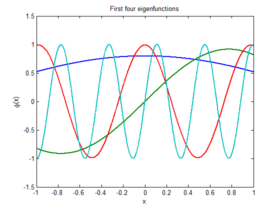
Implemented the Mercem theorem the first four eigenfunction are presented in figure 6 where in figures The Karhunen-Loeve expansion method enables to replace the calculating procedure for the expected value using instead of the abstract space ?? of random fields ? their figures and finally to solve a deterministic problem in space ?? × ?? ? ? ?? instead of space ?? × ??. By performing such replacements in fact a deterministic problem is solved, in contrast to the case of Monte Carlo where a large number of problems carried out. According that the test function of the weak form determined by ?? ? ?? ?? 2 (??, ?? 0 1 (??)) while the solution of the problems in the general form of the boundaries conditions is a function ?? ? ? ?? = ?? ?? 2 (??, ?? ð??"ð??" 1 (??)) which is satisfied the equation:
? ?? ? ?? ?? 2 (??, ?? 0 1 (??))
The expected value of each side assuming that the behavior of source or sink is deterministic and constant:
Where:
?? ? Î?" ? ? is the ? joint density of independent random variables ?
In order to solve the problem according to the finite element method in the current paper we consider a triangle K with nodes ?? ?? ? ?? (??) , ?? (??) ?, ?? = 1,2,3 . To each node N i there is a hat function ?? ?? associated, which takes the value 1 at node ?? ?? and 0 at the other two nodes. Each hat function is a linear function on K so it has the form:
?? i = ?? ?? + ?? ?? ?? + ?? ?? ??(19)The test ?? function belongs to the space:
V h = ????????{?? 1 , ?? 2 , ? , ?? ?? } ? ? 0 1 (D)(20)Any type of higher order shape functions can be used although it will increase the computational cost.
In order to solve the problem of equation 1 we have to create the new space L p 2 (Î?", ? 0 1 (D)). For that reason the subspace S k ? L p 2 (Î?") is considered as (Lord et all 2014).
?? ?? = ????????{ð??"ð??" 1 , ð??"ð??" 2 , ? , ð??"ð??" ? } (21)Using the dyadic product of the space V h , ?? ?? the space L p 2 (Î?", ? 0 1 (D)) created. Thus
?? ??? = ?? ? ??? ?? = ????????{?? ?? ð??"ð??" ?? , i = 1 ? ??, j = 1, ? ??} (22)The space ?? ??? has dimension QN and regards the test function v. In the case where exists ?? ?? finite element supported by boundaries condition then the subspace of solution belongs is:
W hk = V hk ?????????{?? ??+1 , ?? ??+2 , ? , ?? ??+???? } (23)?? ?? ?? = ??? ?? ?? ?? (?? ?? ), ?? ?? = 1,2, ? ???, ?? = 1, ? ??(24)The tensor product of the M ?? ?? ?? subspace results the space of the Generalized Polynomial Chaos:
?? ?? = ?? 1 ??? 2 ? ??? ??(25)Xiu & Karniadakis (2003) show the application of the method for different kind of orthonormal polynomials and in the current paper the Hermite polynomial was used with the following characteristics:
?? 0 = 1, < ?? ?? >= 0, ?? > 0 (26)Where:
?? ?? =< ?? ?? 2 > : are the normalization factors.
?? ???? is the Kronecker delta
??(??) = 1 ?2?? ?? ? ?? 2 is the density function (27)And:
?? ?? = (?1) ?? ?? ?? 2 ?? ?? ???? ?? ?? ? ?? 2 (28)The function ?? ?? ? ?? ??? can be written as the summation of ?? ?? polynomials base as
?? ?? (??, ??) = ? ?? ?? (??)ð??"ð??" ?? (??) ?? ??=1 (29)According that and using the inner product of the weak form equation on each polynomial of the ?? ?? base and get:
< ??????,And let calculate these two integrals:
?? 1 =< ? ?? ???? (??, ??)???(??, ??, ??) ? ???(??)????, ð??"ð??" ?? > ?? = < ? ?? ???? (??, ??) ? ?? ?? (??, ??, ??) nnode i ? ??? ?? (??)??? ?? (??)????, ð??"ð??" ?? > ?? = < ? ?? ?? (??, ??, ??) nnode i ? ?? ???? (??, ??) ? ??? ?? (??)??? ?? (??)????, ð??"ð??" ?? > ?? = < ? ? ?? ?? (??, ??)?? ?? (??) P k nnode i ? ?? ???? (??, ??) ? ??? ?? (??)??? ?? (??)????, ð??"ð??" ?? > ?? = < ? ? ?? ?? (??, ??)?? ?? (??) P k nnode i ? ?? ?? ???? ? (??)+? ??? ?? ?? ?? ?? ?? (??) ?? ??=1 ? ??? ?? (??)??? ?? (??)????, ð??"ð??" ?? > ?? = < ? ? ?? ???? (??, ??)?? ?? (??) P k nnode i ?? ? ??? ?? ?? ?? ?? ?? (??) ?? ??=1 ? ?? ?? ???? ? (??) ? ??? ?? (??)??? ?? (??)????, ð??"ð??" ?? > ?? = ? ? ?? ???? (??, ??) ? ??(??)?? ? ??? ?? ?? ?? ?? ?? (??) ?? ??=1ð??"ð??" ?? (??)ð??"ð??" ?? (??)
?? P k nnode i ? ?? ?? ???? ? (??) ? ??? ?? (??)??? ?? (??)???????? ?? = ?? ?< ?? ??(??) ð??"ð??" ?? (??)ð??"ð??" ?? (??) > ?? ?(??, ??)(36)Where
?? = ? ?? ?? ???? ? (??) ? ??? ?? (??)??? ?? (??)???? ??(37)< ?? ??(??) ð??"ð??" ?? (??)ð??"ð??" ?? (??) > = ? ??(??)?? ? ??? ?? ?? ?? ?? ?? (??)
V.
5. Numerical Example
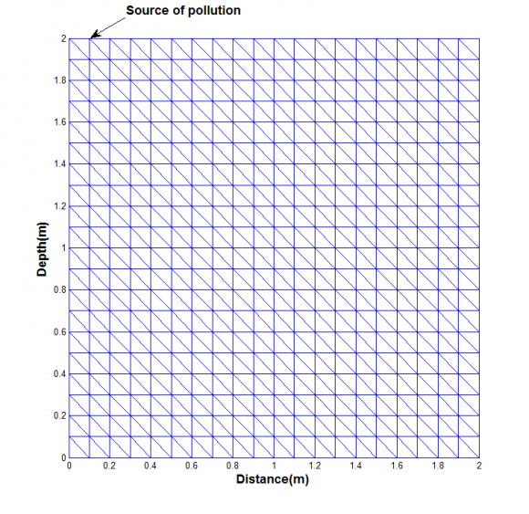
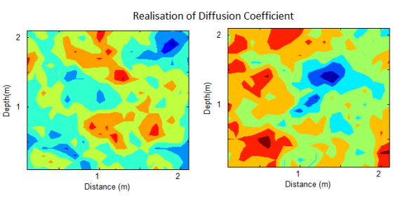
Considering a point source of pollution and the need to estimate its progress due to diffusion and advection phenomena. The problem and the geometry of the finite elements used presented in figure 10. The advection coefficient for simplicity is assumed to be deterministic and constant where the diffusion coefficient present spatial randomness and it is simulated as a random field (figure 11).
To solve the problem the application of the numerical algorithms described in the previous paragraphs is presented and results are compared to those obtained from RFEM using Monte Carlo simulations. The dimensionless input data of the problem is the random field diffusion coefficient with a constant average value equal to 0.1 and a fixed advection coefficient equal to 0.1. An initial source of point pollution equal to 2 is applied as described in figure 10.
In the figures 12-14 the two methods results of the expected values and standard deviation of concentration are shown for variation coefficient ?? ?? = 0.4 and number of Monte Carle samples for the RFEM equal to 1000.
The problem then was solved for three different number of Monte Carle samples for the RFEM and 5, 50, 500 simulations are executed creating 10,100, and 1000 realisation while for SFEM were used one dimensional Hermite GPC with order 3 ( In figures 14, 15 the results for the various calculation are presented. It is observed that as the number of sample increase the results of the Monte Carlo convergence to GPC method and for number of samples equal to 1000 a great accuracy is presented. In figures 17 and 18 this reduction is shown for a variation coefficient ?? ?? = 0.5 .
6. Conclusions
A procedure of conducting a Stochastic Finite Element Analysis of Transport phenomena in Geomechanics where uncertainty arises due to spatial variability of mechanical parameters of soil/rock has been presented. Two different approaches in order to quantifying uncertainty are discussed. The first approach involves generating a random field based on Circulant embedding method and the second Stochastic Finite Element using Polynomial Chaos. A problem of a point source of pollution its progress due to diffusion and advection phenomena used to show the application of the methods.
It is shown that the results of SFEM using polynomial chaos compare well with those obtained from Random Finite Element Method. The main advantage in using the proposed methodology is that a large number of realisations which have to be made for RFEM are avoided, thus making the procedure viable for realistic practical problems. 0.00%
![a) Problem description and Model formulation Let us consider a general spatial domain ?? ? ?? 3 bounded by the surface S. Based on the conservative laws, in the domain, the transport mechanisms, such as convection (also called advection), diffusion can be described by the following equation: ???? (??,??,??) ???? ? ?? ???? (??, ??)???(??, ??, ??) + ??(??, ??)???(??, ??, ??) = ??(??, ??) ???? (0, ??] × ?? × ?? ??(??, ??) = u 0 ???? ?? ?? (1) In order to model the problem assuming the sample space (??, ?, ?) where the ?-algebra is and is considered to contain all the information that is available, is the probability measure. The diffusion and convection coefficient {?? ???? ( ?? , ??) : ? ?? × ??} and the source or sink {??( ?? , ??) : ? ?? × ??} considered as second order random fields and their functions are determined ?? ???? , ??, ??: ?? × ?? ? ? ? ?? = ?? 2 ???, ?? 2 (??)?](https://engineeringresearch.org/index.php/GJRE/article/download/1287/version/101366/3-Stochastic-Finite-Element-Analysis_html/29230/image-2.png)


![Figure 2 : Random field with dimension D = [0,100] × [0,100] and correlation length ? x = ? y = 1 10](https://engineeringresearch.org/index.php/GJRE/article/download/1287/version/101366/3-Stochastic-Finite-Element-Analysis_html/29233/image-5.png)
![?? ?? : are the eigenvalues of the covariance function ?? ?? (??): are the eigenfunctions of the covariance function ??????(?? ?? , ?? ?? ) x ? D and ? ? ? ?? = [?? 1 , ?? 1 , ? , ?? ?? ]: ?? ? ?? ? ? ?? and ?? = ?? 1 × ?? 1 × ? × ?? ?? The pairs of eigenvalues and eigenfunctions arised by the Mercer's theorem: Stochastic Finite Element Analysis for Transport Phenomena in Geomechanics using Polynomial Chaos Global Journal of Researches in Engineering ( ) Volume XV Issue ? ??(?? ?? 2 )??(?? 2 ) = ????(?? 1 ) (15) For two dimensional Domain ?? = [??? 1 , ?? 1 ] × [??? 2 , ?? 2 ] the eigenvalues are ?? ?? = ?? 1 ?? 2 and eigenfunctions are equal to ?? ?? (??) = ?? 1 (?? 1 )?? 2 (?? 2 ) where the values {?? 1 , ?? 2 } and {?? 1 , ?? 2 } calculated by the following equation: ? ??(?? 1 ?? , ?? 2 )?? ?? (?? 2 ) = ?? ?? ?? ?? (?? 1 ), ?? = 1,2 (16)](https://engineeringresearch.org/index.php/GJRE/article/download/1287/version/101366/3-Stochastic-Finite-Element-Analysis_html/29234/image-6.png)

![Figure 6 : First four eigenfunctions in the domain D=[-1,1]](https://engineeringresearch.org/index.php/GJRE/article/download/1287/version/101366/3-Stochastic-Finite-Element-Analysis_html/29236/image-8.png)


![?????? >= ? ??(??) ? ???? ?(??, ??, ?????? >= ? ??(??) ?? [? ?? ???? (??, ??)??? ?(??, ??, ??) ? ???(??)???? ? ?? ? ??(??, ??)??? ?(??, ??, ??) ?? ? ??(??)????]????](https://engineeringresearch.org/index.php/GJRE/article/download/1287/version/101366/3-Stochastic-Finite-Element-Analysis_html/29241/image-13.png)
![?? ??=1 ð??"ð??" ?? (??)ð??"ð??" ?? (??) ?? ???? (38) Stochastic Finite Element Analysis for Transport Phenomena in Geomechanics using Polynomial Chaos Global Journal of Researches in Engineering ( ) Volume XV Issue II Version I ?? ?< ?? ??(??) ð??"ð??" ?? (??)ð??"ð??" ?? (??) > ?? ?(??, ??) (39) And ?? 2 =< ? ??(??, ??)???(??, ??, ??) ?? ? ??(??)????, ð??"ð??" ?? > < ? ??(??, ??) ? ?? ?? (??, ??, ??) nnode i ? ??? ?? (??)?? ?? (??)????, ð??"ð??" ?? ?? , ð??"ð??" ?? > < ? ?? ?? (??, ??, ??) nnode i ? ??(??, ??) ? ??? ?? (??)?? ?? (??)????, ð??"ð??" ?? > ??= < ? ? ?? ?? (??, ??)?? ?? (??) ??, ??) ? ??? ?? (??)?? ?? (??)????, ð??"ð??" ?? > ?? = < ? ? ?? ?? (??, ??)?? ?? (??) P k nnode i ? ?? ??(??)+? ??? ?? ?? ?? ?? ?? (??) ?? ??=1 ? ??? ?? (??)?? ?? (??)????, ð??"ð??" ?? > ?? = < ? ? ?? ???? (??, ??)?? ?? (??) ?? ?? ?? ?? ?? (??) ?? ??=1 ? ?? ??(??) ? ??? ?? (??)?? ?? (??)????, ð??"ð??" ?? > ?? = ? ? ?? ???? (??, ??) ? ??(??)?? ? ??? ?? ?? ?? ?? ?? (??)?? ??=1 ð??"ð??" ?? (??)ð??"ð??" ?? (??) (??) ? ??? ?? (??)?? ?? (??)???????? ?? = ?? ?< ?? ??(??) ð??"ð??" ?? (??)ð??"ð??" ?? (??) > ?? ?(??, ??) (40) Where ?? = ? ?? ??(??) ? ??? ?? (??)?? ?? (??)???? ?? (41) Based on the above the initial equation of the transport phenomena under random behavior is equal to ????(??, ??) ???? ? ?? ?< ð??"ð??" ?? ð??"ð??" ?? > = ?? ?< ?? ??(??) ð??"ð??" ?? (??)ð??"ð??" ?? (??) > ?? ?(??, ??) ? ?? ?< ?? ??(??) ð??"ð??" ?? (??)ð??"ð??" ?? (??) > ?? ?(??, ??) ? ??(??, ??) (42) To solve this system there are various schemes to use and in the current paper the backward Euler method was applied: ???? ? ???? ? ?? ?< ð??"ð??" ?? ð??"ð??" ?? > = ?? ?< ?? ??(??) ð??"ð??" ?? (??)ð??"ð??" ?? (??) > ?? ? ?? ?? +1 ? ?? ?< ?? ??(??) ð??"ð??" ?? (??)ð??"ð??" ?? (??) > ?? ? ?? ?? +1 ? ?? (43) Stochastic Finite Element Analysis for Transport Phenomena in Geomechanics using Polynomial Chaos © 2015 Global Journals Inc. (US) ?< ð??"ð??" ?? ð??"ð??" ?? > (44) ???? = ?? ?< ?? ??(??) ð??"ð??" ?? (??)ð??"ð??" ?? (??) > (45) ???? = ?? ?< ?? ??(??) ð??"ð??" ?? (??)ð??"ð??" ?? (??) > (46) ???? ? ???? ? ???? = ?????? ? ?? ?? +1 ? ?????? ? ?? ?? +1 ? ?? (47) After some algebra: ?? ? ?? ?? +1 = ?????? ? ?? ?? ? ???? ? ?? ???? ? ????(???? ? ????) (48) The statistical moments of the displacement field arise by the properties of the Polynomial of Chaos expansion: The expected value ?? 0 (??)ð?"¼ð?"¼[ð??"ð??" 0 (??)] ??????????? ? ?? ?? (??)ð?"¼ð?"¼[ð??"ð??" ?? (??)] ?? 0 (??) (49) And the variance ?? 2 = ð?"¼ð?"¼(??(??, ??) ? ð?"¼ð?"¼[??(??, ??)]) 2 = ð?"¼ð?"¼(? ?? ?? (??)ð?"¼ð?"¼[ð??"ð??" ?? (??)] ? ?? 0 (??)) ? ?? ??=0 ?? 2 = ? ?? ?? 2 (??)ð?"¼ð?"¼?ð??"ð??" ?? 2 ? ?? ??=0](https://engineeringresearch.org/index.php/GJRE/article/download/1287/version/101366/3-Stochastic-Finite-Element-Analysis_html/29242/image-14.png)


| c) Generalized Polynomial of chaos and stochastic | ||||
| Galerkin solution | ||||
| Assuming that the ?? ?? ?? represents a space | ||||
| of | univariate | orthonormal | polynomial | of |
| variable ?? ?? ? ?? ?? ? ? with order k or lower and: | ||||
| ( ) Volume XV Issue | ||||
| Global Journal of Researches in Engineering | ||||
| ? | |||||||
| ?? | |||||||
| ?< ? ??(??, ??)???(??, ??, ??) | ? ??(??)????, ð??"ð??" ?? > ? ? ??(??, ??) ? ??(??)???? | (33) | |||||
| ?? | ?? | ||||||
| Set | |||||||
| ?? 1 =< ? ?? ???? (??, ??)???(??, ??, ??) ? ???(??)????, ð??"ð??" ?? > | (34) | ||||||
| ?? | |||||||
| Year 2015 | ?? ?? 2 < ? ??(??, ??)???(??, ??, ??) | ? ??(??)????, ð??"ð??" ?? > | |||||
| 40 | |||||||
| I | |||||||
| Global Journal of Researches in Engineering E ( ) Volum e XV Issue II Version | Where: | ð??"ð??" ?? >=< ? ?? < ? ???? ?? ? ???? ??=1 ?? ???? (? ?? ?? ?? ? ?? ?? ? ?? ?? ???? ? ? < ? ?????????? ???? ???? (??, ??) ???? ?? ?????????? ??=1 ? ? ???? ???? (??, ??) ???? ?? ? ??(??)ð??"ð??" ?? (??)ð??"ð??" ?? (??) ? ?? ?? (??)????, ð??"ð??" ?? >= ?? ?? ??=1 ? ?? ?? (??) ? ?? ?? (??)???????? ?? ?????????? ??=1 ????(??, ??) ???? ? ??? < ð??"ð??" ?? ð??"ð??" ?? > ??=1 ? ?? ?? ?????????? | = | (30) | |||
| ?? = ? ?? ?? (??) ? ?? ?? (??) | ???? | (31) | |||||
| ?? | |||||||
| 16.00% |
| 14.00% |
| 12.00% |
| 10.00% |
| 8.00% |
| 6.00% |
| 2.00% 4.00% Î?"std[uGlobal Journal of Researches in Engineering 1 10 100 1000 ( ) Volume XV Issue II Version I |