1. Introduction
obotics is the science that deals with robot's design, modeling and controlling. Nowadays robots are used everywhere in everyday life. It has accompanied people in most of industry and daily life jobs. (Gouasmi, Ouali, Fernini, & Meghatria, 2012).
The range of robot utilization is very wide. A large family of robots is used in industry and manufacturing. Robots are used in supplying the motion required in manufacturing processes such as pick and place, assembly, painting, milling, cutting, welding, drilling, etc.
Because of different types of tasks different manipulator configurations are available such as rectangular, cylindrical, spherical, revolute and horizontal jointed (Gouasmi et al., 2012).
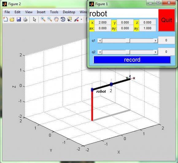
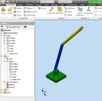
A two revolute joint robot configuration with two degrees of freedom is generally well-suited for small parts insertion and assembly, like electronic components. Although the final goal is to design and manufacture real robotics, it is very useful to perform simulations prior to investigations with real robots. Simulations are easier to setup, less expensive, faster and more convenient to use. it allows better design exploration and helps you enhance your final real robot by selecting suitable parameters for the system you want to design (?lajpah, 2008).
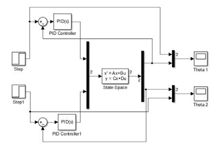
There are many control techniques used to control a robot arm. The most used ones are the PID control, optimal control, adaptive control and robust control. "There are many kinds of controllers that can be used to cause a designed robot arm to move along a desired trajectory" (Sukvichai, 2008). The simplest which we used in this paper to control the robot arm is the PID controller. The (D-H) parameters for the 2-R robot will be defined as in the table below. The initial position (at t = 0) from the homogeneous transformation matrix where ? 1 = 0 °?2 = 0 ° are shown in figure (2).
2. II.
3. Problem Formulation
4. Robot Dynamics
Description of x and y in terms of ? 1 and ? 2 in term of linear displacement:
?? 1 =?? 1 sin?? 1 ?? 1 =?? 1 cos?? 1 ?? 2 =?? 1 sin?? 1 +?? 2 sin (?? 1 +?? 2 ) ?? 2 =?? 1 cos?? 1 +?? 2 cos (?? 1 +?? 2 )So, Kinetic Energy could be formed as:
KE = 1 2 m 1 v 1 2 + 1 2 m 2 v 2 2 + 1 2 j 1 ? 1 2 + 1 2 j 2 ? 2 2 (1)Substitute for v1 and v2
KE 1 2 m 1 l g1 2 ? ?1 + 1 2 m 2 ?l 1 2 ? ?1 + 2l 1 l g2 ? ?1? ? ?1 + ? ?2? cos ? 2 + l g2 2 ? ? ?1 + ? ?2? 2 ? + 1 2 j 1 ? ?1 + 1 2 j 1 ? ? ?1 + ? ?2? 2 (2)And Potential Energy is
PE = m 1 gl g1 sin? 1 + m 2 g(l 1 sin? 1 + (l g2 sin (? 1 + ? 1 ))(3)a) Equations of motion
The Lagrangian of a dynamic system is defined as the difference between the kinetic and potential energy at an arbitrary instant (N.Jazar, 2010).
5. L = KE ? PE So, by Lagrange Dynamics, we form the Lagrangian
Using Lagrange to form generalized equations of motion in matrix form as:
? m 1 l g1 2 + m 2 l 1 2 + j 1 m 2 l 1 l g2 cos(? 1 ? ? 2 ) m 2 l 1 l g2 cos(? 1 ? ? 2 ) m 2 l g2 2 + j 2 ? ? ? 1 ? 2 ?? ? ?m 2 l 1 l g2 g sin(? 1 ? ? 2 ? ? ? 1 ? 2 ?? + ? (m 1 l g1 + m 2 l 1 ) g cos? 1 m 2 l g2 g cos? 2 ? = ? M 1 M 2 ? (5)And the general form is:
H(q?) + C (q? , q) + g(q) = M IV.6. Pid Controller based on Linear Model
We define new variables in order to convert the 2-R robot to an equivalent linear model.
x 1 = ? 1 x 2 = ? 2 x 3 = ? 1 ?x4 = ? 2 ? ???1 = ? 1 ?= x 3 ???2 = ? 2 ?= x 4 ???3 = ? 1 ????4 = ? 2 ?Rewrite the equation of motion using these variables, and use new constants c 1 to c 6 function of robot specifications to make equations in simple form
x 4 ?= M 2 c 5 ? c 2 M 2 c 5 cos(x 1 ? x 2 ) + c 3 c 5 sin(x 1 ? x 2 ) x 4 ? c 6 c 5 cos x 2 (6) ?c 1 ? M 2 c 5 cos 2 (x 1 ? x 2 )? x 3 ?= M 1 ? c 2 M 2 c 5 cos(x 1 ? x 2 ) ? c 2 c 3 c 5 cos(x 1 ? x 2 ) sin(x 1 ? x 2 ) x 4 + c 2 c 6 c 5 cos(x 1 ? x 2 ) cosx 3 ? c 4 cos x 1(7)x 1 ?= x 3 (8)
x 2 ?= x 4(9)Y=?
1 0 0 0 0 1 0 0 0 0 1 0 0 0 0 1 ? ? ? x 1 ? x 2 ? x 3 ? x 4 ? + [0][D] a) Linearized modelWe substitute values of constants c 1 to c 6 into the state-space model to get the state space matrices:
7. H
Now we can write the state-space model using linearization about the equilibrium point:
? 1 = ? ? 2 ? 1 ?= 0? 2 = ? ? 2 ? 2 ?= 0 M1= 0 M2= 0We Perform Taylor series expansion of the nonlinear functions and neglect high-order terms, to get the linearized model. At equilibrium point: Linearization of the variable x 1 with respect to other variables:
?x 1 ?x 1 = 0 ?x 1 ?x 2 = 0 ?x 1 ?x 3 = 1 ?x 1 ?x 4 = 0Linearization of the variable x 1 with respect to other variables:
?x 2 ?x 1 = 0 ?x 2 ?x 2 = 0 ?x 2 ?x 3 = 0 ?x 2 ?x 4 = 1Linearization of the variable x 1 with respect to other variables: Linearization of the variable x 1 and x 2 with respect to input torques:
?x 1 ?M 1 = 0 ?x 1 ?M 2 = 0 ?x 2 ?M 1 = 0 ?x 2 ?M 2 = 0 ?x 3 ?M 1 = c 5 c 1 c 5 ? M 2 ?x 3 ?M 2 = ? c 2 c 1 c 5 ? M 2 ?x 4 ?M 1 = 0 ?x 4 ?M 2 = 1 ? c 2 c 5We can write the state-space model:
? ?x 1 ?x 2 ?x 3 ?x 4 ?? = ? ? ? ? ? ? 0 0 c 4 c 5 c 1 c 5 ? M 2 0 0 0 c 2 c 6 c 1 c 5 ? M 2 ? c 6 c 5 1 0 0 0 0 1 0 0 ? ? ? ? ? ? ? ? x 1 ? x 2 ? x 3 ? x 4 ? + ? ? ? ? ? ? 0 0 c 5 c 1 c 5 ? M 2 0 0 0 ? c 2 c 1 c 5 ? M 2 1 ? c 2 c 5 ? ? ? ? ? ? ? ? M 1 ? M 2 ?8. Pid Controller based on Feedback Linearization
Having system's equation H(q?) + C (q? , q) + g(q) = M q?= H ?1 [? C (q? , q) ? g(q)] + M ? While:
M ? = H ?1 MAnd, M = H ?1 M ?This way, we decoupled the system to have the (non-physical) torque input:
M ? = H ?1 ? M 1 M 2 ?However, the physical torque inputs to the system are:
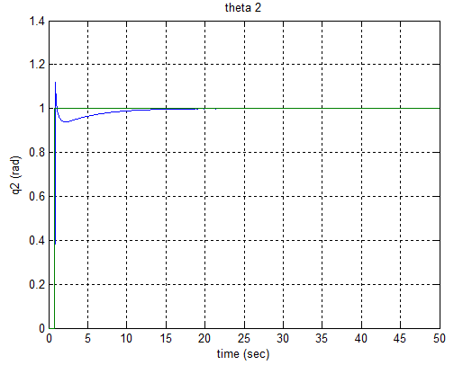
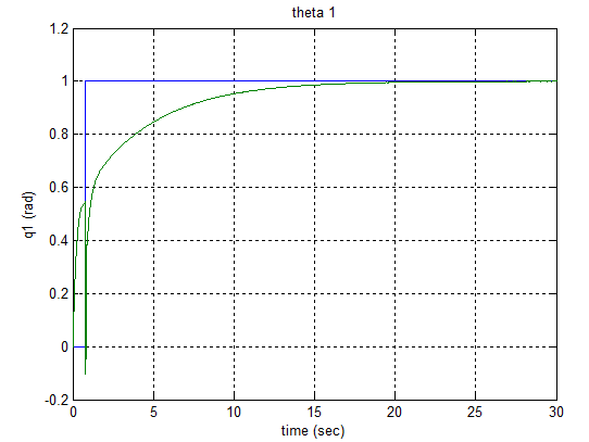
M = H ? M ? 1 M ? 2 ?To design the feedback PID controller, error signals are assumed to be: We notice that the response is following the control signal with relatively good manner. And errors of ? 1 and ? 2 are equal to zero in a short time.
9. VII.
10. Conclusion
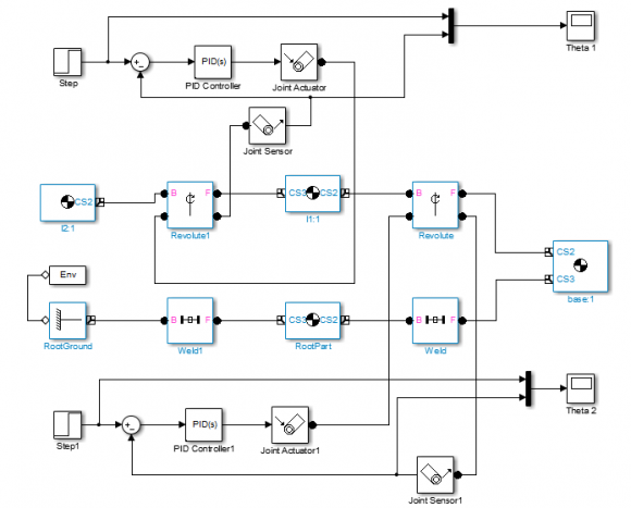
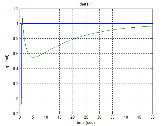
The main content of this paper is about modeling a 2-R robotusing two methods: first is mathematical modeling using Lagrange dynamic equations and the second is using Autodesk Inventor and Simulink software's to develop the model. After that we used PID controller to validate the models and to notice the difference in accuracy achieved by each technique. Linearization about working point is valid in one point only, while it is no longer valid for other points. The model designed from Autodesk Inventor and Simulink software's is giving better and reasonable response. Good results are found when using feedback linearization.

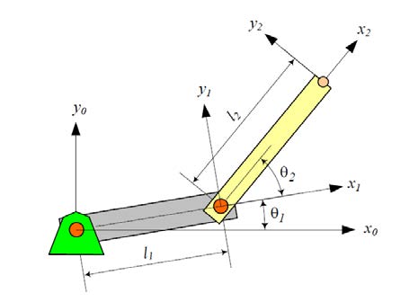


| D-H parameters of 2-R Robot | ||||
| Frame No. | ?? ?? | ?? ?? | ?? ?? | ?? ?? |
| 1 | L 1 | 0 | 0 | ? 1 |
| 2 | L 2 | 0 | 0 | ? 2 |