1. Introduction
ourier analysis occurs in the modeling of timedependent phenomena that are exactly or approximately periodic. Examples of this include the digital processing of information such as speech; the analysis of natural phenomen such as earthquakes; in the study of vibrations of spherical, circular or rectangular structures; and in the processing of images. In a typical case, Fourier spectral methods write the solution to the partial differential equation as its Fourier series. Fourier series decomposes a periodic realvalued function of real argument into a sum of simple oscillating trigonometric functions (??????????, ??????????????), that can be recombined to obtain the original function. Substituting this series into the partial differential equation gives a system of ordinary differential equations for the time-dependent coefficients of the trigonometric terms in the series then we choose a timestepping method to solve those ordinary differential equations II.
2. Fourier Series
The Fourier series of a smooth and periodic real-valued function ð??"ð??"(??) ? [0; 2??] with period 2?? is
L x n x f L a L n ) sin( ) ( 1 2 0 ? ? = .... 2 , 1 , 0 = n (2) dx L x n x f L b L n ) cos( ) ( 1 2 0 ? ? = .... 2 , 1 = n (3)Fourier series can be expressed neatly in complex form as follows
? ? = ? ? ? ? ? ? ? ? ? ? ? ? ? ? ? + ? ? ? ? ? ? + + = 1 2 2 2 f(x) n L x in L x in n L x in L x in3. Discrete Fourier Transform
In many applications, particularly in analyzing of real situations, the function ( ) f x to be approximated is known only on a discrete set of "sampling points" of x. Hence, the integral (7) cannot be evaluated in a closed form and Fourier analysis cannot be applied directly. It then becomes necessary to replace continuous Fourier analysis by a discrete version of it. The linear discrete Fourier transform of a periodic (discrete) sequence of complex values ?? 0 , ?? 0 , ? , ?? ?? ?? ?1 with period ?? ?? ?? , is a sequence of periodic complex values ?? ? 0 , ?? ? 1 , ? , ?? ? ?? ?? ?1 defined by
? ? = ? = 1 0 2 k 1 u ~? ? ? ? N j N k ij j e u N (8)The linear inverse transformation is
? ? = = 1 0 2 k j u ? ? ? ? N k N k ij e (9)The most obvious application of discrete Fourier analysis consists in the numerical calculation of Fourier coefficients. Suppose we want to approximate a realvalued periodic function ( ) f x defined on the interval [0; 2??] that is sampled with an even number N ? of grid
points jh = j x ? N 2L h = 1 N 0,1,...., j ? = ? (10)by it is Fourier series. First we compute approximate values of the Fourier coefficients
? ? = ? ? 1 0 2 k ) ( 1 c ~? ? ? ? N j N k ij e x f N (11)Because the discrete Fourier transform and its inverse exhibit periodicity with period ?? ?? , i.e. ?? ? ?? + ?? ?? = ?? ? ?? (this property results from the periodic nature of ?? 2???????? ?? ?? ), it makes no sense to use more than ?? ?? terms in the series, and it suffices to calculate one full period. The Fourier series formed with the approximate coefficients is
? + ? = ? ? 2 / 1 2 / 2 ) ( f ~?? ? ? N N k N k ij k e c x (11')The function ð??"ð??" ?(??) not only approximates, but actually interpolates ð??"ð??"(??) at the sampling grid points ?? ??
In matrix form, the discrete Fourier transform (8) can be written as
j kj u M N ? 1 u ~k= 1 ,... 1 , 0 , ? = ? N j k (12)Where
? kj kj M = and ? ? ? N i e 2 ? = ? ? ? ? ? ? ? ? ? ? ? ? ? ? ? ? = 1) - 1)(N - (N 1) - 2(N 1 - N 1) - 3(N 1) - 2(N 1 - N 6 4 2 3 2 1 1 1 1 1 1 1 1 ? ? ? ? ? ? ? ? ? ? ? ? ? ? ? ? ? ? ? ? ? ? ? ? ? ? ? ? ? M Similarly, the inverse discrete Fourier transform has the form k * j u ? kj M = 1 ,... 1 , 0 , ? = ? N j k (13) Where * * ? kj kj M = and ? ? ? N i e 2 * = where ð??"ð??" * is complex conjugate of ð??"ð??" ? ? ? ? ? ? ? ? ? ? ? ? ? ? ? ? = 1) - 1)(N - (N * 1) - 2(N * 1 - N * 1) - 3(N * 1) - 2(N * 1 - N * 6 * 4 * 2 * 3 * 2 * * * 1 1 1 1 1 1 1 1 ? ? ? ? ? ? ? ? ? ? ? ? ? ? ? ? ? ? ? ? ? ? ? ? ? ? ? ? ?4. M
The FFT algorithm reduces the computational work required to carry out a discrete Fourier transform by reducing the number of multiplications and additions of (13) , computational time is reduced from ??(?? 2 ?? ) to ??(?? ?? log ?? ?? ).
To apply spectral methods to a partial differential equation we need to evaluate derivatives of functions. Suppose that we have a periodic real-valued function ( ) f x ? [0; 2??] with period 2?? that is discretized I with an even number N ? of grid points, so that the grid size ? N 2L h = .The complex form of the Fourier series representation of ( )
f x is /2 /2 1 f ( ) N i kx L k k N x c e ? ? ? = ? + ? ? ? ? At 2 N k ? =the above series gives a term , and since it cannot be differentiated, we should set its derivative to be zero at the grid points. The numerical derivatives of the function ( ) f x can be illustrated as a matrix multiplication.For the first derivative, we multiply the Fourier coefficients (11) by the corresponding differentiation matrix for an even number N ? of grid points.
N N i Diag L ? ? ? ? ? ? ? ? = ? ? ? ? ? ? ? ? ? ? ? ? ? ?This matrix has non-zero elements only on the diagonal. For an odd number N ? of grid points the differentiation matrix corresponding to the first derivative is diagonal with elements.
0,1, 2,3...., 1, 0, 1 ,...., 3 2 1 2 2
N N i L ? ? ? ? ? ? ? ? ? ? ? ? ? ? ? ? ? ? ? ? ?Then, we compute an inverse discrete Fourier transform using (11 ? ) to return to the physical space and deduce the first derivative of f (x) on the grid. Similarly, taking the second derivative corresponds to the multiplication of the Fourier coefficients (11) by the corresponding differentiation matrix for an even number N ? of grid points.
N N N i Diag L ? ? ? ? ? ? ? ? ? ? ? ? ? ? ? = ? ? ? ? ? ? ? ? ? ? ? ? ? ? ? ? ? ? ? ? ? ? ? ?In general, in case of an even number N ? of grid points approximating the m -th numerical derivatives of a grid function ( ) f x corresponds to the multiplication of the Fourier coefficients (11) by the corresponding differentiation matrix which is diagonal with elements
m ik L ? ? ? ? ? ? ? for 0,1, 2,3...., 1, , 1 ,...., 3 2 1 2 2 2 N N N k ? ? ? ? ? = ? ? ? ? ? ? ? ? ? ?with the exception that for odd derivatives we set the derivative of the highest mode
5. Exponential Time Differencing
The family of exponential time differencing schemes. This class of schemes is especially suited to semi-linear problems which can be split into a linear part which contains the stiffest part of the dynamics of the problem, and a nonlinear part, which varies more slowly than the linear part. Exponential time differencing schemes are time integration methods that can be efficiently combined with spatial approximations to provide accurate smooth solutions for stiff or highly oscillatory semi-linear partial differential equations.In this paper I will present the derivation of the explicit Exponential time differencing schemes for arbitrary order following the approach in [ ] [ ] [ ]
t t = to t t t t n n ? + = = +1 to obtain. ? ? ? d t t u F t u t u t n n t c t c n n e e ? ? ? ? + + + + = 0 1 ) ), ( ( * ) ( ) ( (?? 1 )The next step is to derive approximations to the integral in equation (?? 1 ). This procedure does not introduce an unwanted fast time scale into the solution and the schemes can be generalized to arbitrary order.
If we apply the Newton Backward Difference Formula, we can write a polynomial approximation to ) ), ( (
? ? + + n n t t u F in the form ( ) ( ) ? ? ? ? ? ? ? ? ? ? ? ? ? ? ? ? ? ? ? ? ? ? ? = ? = ? ? ? ? ? ? ? ? ? = ? ? ? ? ? ? ? ? ? ? ? ? ? ? ? ? ? ? ? ? ? ? ? ? ? ? ? ? ? ? ? ? ? ? ? = ? + + ? ? ? n t G m t t u F k m m t n t G m m t t t G t t u F n k n k n m k m s m m n s m m n n n ), ( ) 1 ( * / ) 1 ( * / ) 1 ( , ) ), ( ( 0 1 0 1 0 ? ? ? ? (?? 2 ) 1 ,..., 1 ), 1 )...( 2 )( 1 ( ! ? = + ? ? ? = ? ? ? ? ? ? ? ? s m k m m m k m k note that 1 0 ! 0 = ? ? ? ? ? ? ? ? m If we substitute (?? 2 ) into (?? 1 ) we get ? ? d n t G m m t t u t u t n s m m t c t c n n e e ? ? ? ? ? ? ? ? ? ? ? ? = ? ? + ? ? ? ? ? ? ? ? ? ? ? ? + = 0 1 0 1 * / ) 1 ( * ) ( ) ( ) / ( * / * ) 1 ( ) ( ) ( 1 0 ) / 1 ( 1 0 1 t d n t G m m t t t u t u n t t c s m m t c n n e e ? ? ? ? ? ? ? ? ? ? ? ? ? ? = ? ? ? ? ? ? ? ? ? ? ? ? ? ? ? = ? + ? ? ? (?? 3 )We will indicate the integral by
) / ( / 1 0 ) / 1 ( t d m t e t t c m ? ? ? ? ? ? ? ? ? ? ? = ? ? ? ? ? ? ? ? (?? 4 )If we substitute (?? 2 ) and (?? 4 ) into (?? 3 ) we get ( )
k n k n m k m s m m m t c n n t t u F k m t t u t u e ? ? = ? = ? + ? ? ? ? ? ? ? ? ? ? ? ? ? + = ), ( ) 1 ( * * ) 1 ( ) ( ) ( 0 1 0 1 ? (?? 5 )Which represent the general generating formula of the exponential time differencing schemes of order s The first-order exponential time differencing scheme is obtained by setting s=1
c F u u n t c t c n n e e / ) 1 ( 1 ? + = ? ? +The second-order exponential time differencing scheme is obtained by setting s=2
{ } ) /( ) 1 ( ) 1 2 ) 1 (( 2 1 1 t c F t c F t c t c u u n t c n t c t c n n e e e ? + ? + ? + ? ? ? + ? + = ? ? ? ? +6. ?
By setting s=2 we get the fourth-order exponential time differencing scheme
) 6 /( ) ( 3 4 3 4 2 3 1 2 1 1 t c F F F F u u n n n n t c n n e ? ? ? + ? ? ? + = ? ? ? ? + 6 18 2611 24 ) 6 12 11 6 ( 2 2 3 3 2 2 3 3 1 ? ? ? ? ? ? ? + ? + ? + ? = ? ? t c? = ? + ? + ? ? ? ? ? ? ? . I V.On the Stability of Etdrk4 Method
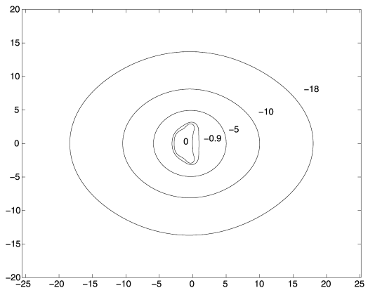
The stability analysis of the ETDRK4 method is as follows (see [21,24] , , , , ? ? ? ? ? by the above expressions suffers from numerical instability for y close to zero. Because of that, for small y , instead of them, we will use their asymptotic expansions. ? Because c and ? may be complex, the stability region of the ETDRK4 method is four-dimensional and therefore quite difficult to represent. Unfortunately, we do not know any expression for ( , ) 1 r x y = we will only be able to plot it. The most common idea is to study it for each particular case; for example, assuming c to be fixed and real in [21] or that both c and ? are pure imaginary numbers in [24]. For dissipative PDEs with periodic boundary conditions, the scalars c that arise with a Fourier spectral method are negative. Let us take for example Burger's equation
2 1 ( ) 2 t xx x u u u ? = ? [ , ] x ? ? ? ?where 0 1 ? < ? (3.4) Transforming it to the Fourier space gives In Figure . 1 we draw the boundary stability regions in the complex plane x for y=0,-0.9,-5,-10,-18 .
When the linear part is zero ( 0 y = ), we recognized the stability region of the fourth-order Runge-Kutta methods and, as y ?? ?
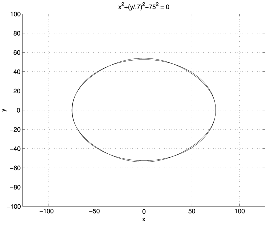
, the region grows. Of course, these regions only give an indication of the stability of the method. In 0 y < , 1 y << the boundaries that are observed approach to ellipses whose parameters have been fitted numerically with the following result. x = , the intersection with the imaginary axis Im( )
x increases as y , i.e., as 2
? .Since the boundary of stability grows faster than , the ETDRK4 method should have a very good behavior to solve Burger's equation, which confirms the results of paper [6].
VI.
7. Exponential Time Differencing Runge-Kutta Methods
Generally, for the one-step time-discretization methods and the Runge-Kutta methods, all the information required to start the integration is available.However, for the multi-step time-discretization methods this is not true.These methods require the evaluations of a certain number of starting values of the nonlinear term ) ), ( ( t t u F at the n -th and previous time steps to build the history required for the calculations.Therefore, it is desirable to construct exponential time differencing methods that are based on Runge-Kutta methods.
8. Based in [ ]
12 and [ ]
= + ? ? ? + ? ? ? + ? ? + ? + + ? + + ? ? ? + ? ? + ? ? ? + ? ? (?? 12 )In general, the exponential time differencing Runge-Kutta method (?? 12 ) has classical order four, but Hochbruck and Ostermann [11] showed that this method suffers from an order reduction. They also presented numerical experiments which show that the order reduction, predicted by their theory, may in fact arise in practical examples. In the worst case, this leads to an order reduction to order three for the Cox and Matthews method (?? 12 ) [12] . However, for certain problems, such the numerical experiments conducted by Kassam and Trefethen [13] , [6] for solving various one-dimensional diffusion-type problems, and the numerical results obtained in for solving some dissipative and dispersive PDEs, the fourth-order convergence of the fourth-order Runge Kutta exponential time differencing method [12] is confirmed numerically.
Finally, we note that as 0 c ? in the coefficients of the s -order exponential time differencing Runge-Kutta methods, the methods reduce to the corresponding order of the Runge-Kutta schemes.
V.
9. The Kuramoto-Sivashinsky Equation
The Kuramoto-Sivashinsky equation,is one of the simplest PDEs capable of describing complex behavior in both time and space. This equation has been of mathematical interest because of its rich dynamical properties. In physical terms, this equation describes reaction diffusion problems, and the dynamics of viscousfuid films flowing along walls.
Kuramoto-Sivashinsky equation in one space dimension can be written
4 42 2 ) , ( ) , ( ) , ( ) , ( ) , ( x tx u x t x u x t x u t x u t t x u ? ? ? ? ? ? ? ? ? = ? ? (14)Equation ( 14) can be written in integral form if we introduce
t t x t x u ? ? = ) , ( ) , ( ? then 4 4 2 2 2 ) , ( ) , ( ) , (21 ) , ( x t x x t x x t x t t x ? ? ? ? ? ? ? ? ? ? ? ? ? ? ? = ? ? ? ? ? ? (15) or in form 0 2 / 2 2 4 = + + + ? ? ? u u u utThe Kuramoto-Sivashinsky equation with 2?? periodic boundary conditions in Fourier space can be written as follows 14) can be written as fellows ( )
? ? = = 1 0 ) ( ? ? N k L x ik k j e u x u? ? ? ? ? ? ? ? ? ? ? ? ? ? ? ? ? ? ? ? ? ? ? ? ? ? ? ? ? ? ? ? ? ? ? ? ? ? ? ? ? ? ? ? ? ? ? ? ? ? ? ? ? = â??" ? ? ? ? ? ? ? ? ? = ? ? â??" ? ? ? ? ? ? ? ? ? = ? ? ? ? ? ?= ? = , 1 4 , 1 2 = ? = ? ? ? ? ? ? ? ? ? ? ? ? i i ? N L h jh j x 2 , = = Equation (? k k k ik t u t t u k k 2 ) ( ) ( ~4 2 ? ? = ? ? (17) Where = = ? ? dx t x u L L L L x ik k e ? ? ) , (21 2 [ ] 2 / 2 1 0 ) ( ) , ( 2 1 t u FFT e t x N N ijk N j j u = ? ? = ? ? ?In final form will be (
)
[ ] 2 4 2 ) ( 2 ) ( ) ( ~t u FFT ik t u t t u k k k k ? ? = ? ? (18)Equation has strong dissipative dynamics, which arise from the fourth order dissipation The stiffness in the system (17) is due to the fact that the diagonal linear operator ( )
k k 4 2 ?, with the elements, has some large negative real eigenvalues that represent decay, because of the strong dissipation, on a time scale much shorter than that typical of the nonlinear term. The nature of the solutions to the the Kuramoto-Sivashinsky equation varies with the system size of linear operator. For large size of linear operator, enough unstable Fourier modes exist to make the system chaotic. For small size of linear operator, insuffcient Fourier modes exist, causing the system to approach a steady state solution. In this case, the exponential time differencing methods integrate the system very much more accurately than other methods since the the exponential time differencing methods assume in their derivation that the solution varies slowly in time.
VI.
10. Numerical Result
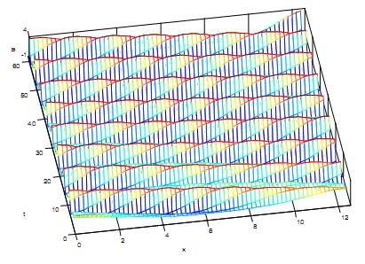
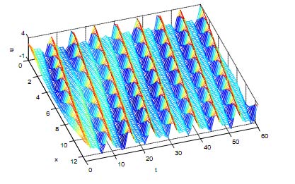
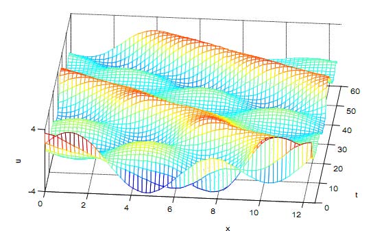
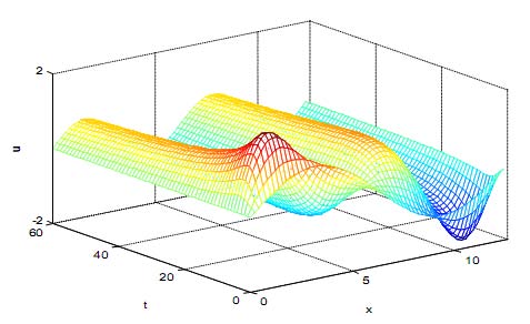
For the simulation tests, we choose two periodic initial conditions
[ ] ? 4 , 0 , ) ( 2 cos 1 ? = ? ? ? ? ? ? x x u e x [ ] ? 4 , 0 ), sin( 4 . 2 ) cos( 6 . 0 2 sin 1 . 0 2 cos 7 . 1 ) ( 2 ? + + ? ? ? ? ? ? + ? ? ? ? ? ? = x x x x x x uWhen evaluating the coefficients of the exponential time differencing and the exponential time differencing Runge Kutta methods via the "Cauchy integral" approach , the solution appears more clear as a mesh plot and shows waves propagating, traveling periodically in time and persisting without change of shape.
11. VII.
12. Conclusions
In this paper, the main objective of this study was for finding the solution of one dimensional semilinear fourth order hyperbolic Kuramoto-Sivashinsky equation, describing reaction diffusion problems, and the dynamics of viscous-fuid films flowing along walls. In order to achieve this, we applied Fourier spectral approximation for the spatial discretization. In addition, we evaluated the coeffcients of the exponential time differencing and the exponential time differencing -fourth order Runge Kutta methods via the "Cauchy integral" .Some typical examples have been demonstrated in order to illustrate the efficiency and accuracy of the exponential time differencing methods technique in this case. For the simulation tests, we chose periodic boundary conditions and applied Fourier spectral approximation for the spatial discretization. In addition, we evaluated the coefficients of the Exponential Time Differencing Runge-Kutta methods via the "Cauchy integral" approach. The equations can be used repeatedly with necessary adaptations of the initial conditions.

| ( ) du t cu t ( ) dt = | + | ? | ( ) u t | (3.2) | |||||||||||||||||||||||||||||||||||||||||||||||||||||||
| and the fixed point 0 ( ) u t is stable if Re( | ) 0 + < . c ? | ||||||||||||||||||||||||||||||||||||||||||||||||||||||||||
| ( dt t du | ) | = | cu | ( t | ) | + | F | ( u | ( t | ), | t | ) | (3.1) | The application of the ETDRK4 method to (3.2) leads to a recurrence relation involving n u and 1 n u + . | |||||||||||||||||||||||||||||||||||||||||||||
| with | ( ( ), ) F u t t the nonlinear part, we suppose | Introducing the previous notation x | = | ? | h | and y ch = , | |||||||||||||||||||||||||||||||||||||||||||||||||||||
| that there exists a fixed point 0 u this means that | and using the Mathematica © algebra obtain the following amplification factor | package, we | |||||||||||||||||||||||||||||||||||||||||||||||||||||||||
| 0 cu F u t 0 ( , ) 0 + = . Linearizing about this fixed point, if ( ) u t is the perturbation of 0 u and 0 '( , ) F u t ? = then | 1 + = n n r x y ( , ) u u | 0 = + ? ? | 1 | x | + | ? | 2 | x | 2 | + | ? | 3 | x | 3 | + | ? | 4 | x | 4 | (3.3) | |||||||||||||||||||||||||||||||||||||||
| where | |||||||||||||||||||||||||||||||||||||||||||||||||||||||||||
| ? | 0 | = | e | y | |||||||||||||||||||||||||||||||||||||||||||||||||||||||
| y | 3 | y | y | 3 | y | ||||||||||||||||||||||||||||||||||||||||||||||||||||||
| ? | 1 | = | 2 3 e 4 8 3 y y ? + | ? | 8 e y | 2 3 | + | 4 e y | 2 3 | y | 2 2 e y 1 4 2 y ? + | ? | 2 y e y 6 | + | 4 y e | 2 2 | ? | 2 2 y y e | |||||||||||||||||||||||||||||||||||||||||
| y | 3 | y | y | 3 | y | y | |||||||||||||||||||||||||||||||||||||||||||||||||||||
| ? | 2 | 4 8 16 y y e 4 ? = + | 2 | ? | 4 e y 16 | 2 | + | 8 e y | 2 4 | y | 3 5 12 y y e 3 ? + | 2 | ? | 3 e y 10 | y | + | 4 | e y | 2 3 | ? | 2 3 y y e | ? | 2 2 e y 1 4 2 y + | ? | 3 3 , y e y | ||||||||||||||||||||||||||||||||||
| ? | 3 | 5 4 16 e 5 y y = ? | y 2 | + | 5 e 16 y | y | + | 8 e y | 3 2 y 5 | ? | 2 5 e 20 y | y | + | 5 5 y e 8 | y 2 | ? | 4 2 y | + | 4 10 e y ? | y 2 | + | 4 e y 16 | y | ? | 3 2 y 4 e y 12 | + | 6 y e | 2 4 | y | ? | 2 y e | 5 4 | y 2 | ||||||||||||||||||||||||||
| ? | y 2 3 e 2 y | + | 3 y e 4 y | ? | 2 e y | 3 3 | y 2 | ||||||||||||||||||||||||||||||||||||||||||||||||||||
| ? | 4 | = | 6 8 24 e 6 y y ? | y 2 | + | 6 e 16 y | y | + | 3 2 y 5 e 16 y | ? | 2 6 e 24 y | y | + | 5 6 y e 8 | y 2 | 5 6 y + + | 5 18 e y ? | y 2 | + | 5 e y 20 | y | ? | 3 2 y 5 e y 12 | + | 6 y e | 2 5 | y | + | 2 | e y | 5 5 | y 2 | |||||||||||||||||||||||||||
| y 2 4 e 2 6 4 y y + ? | + | 4 y e 6 y | ? | 2 e y | 3 4 | y 2 | |||||||||||||||||||||||||||||||||||||||||||||||||||||
| An | important | remark: | computing | ||||||||||||||||||||||||||||||||||||||||||||||||||||||||
| 0 | 1 | 2 | 3 | 4 | |||||||||||||||||||||||||||||||||||||||||||||||||||||||