cceleration is one form of determining a vehicle's performances.

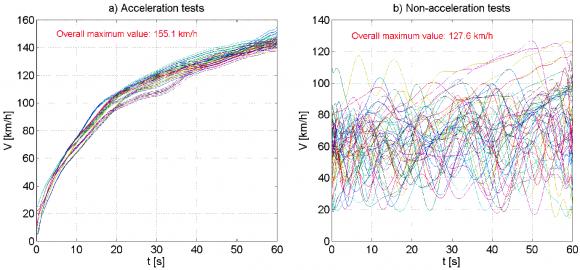
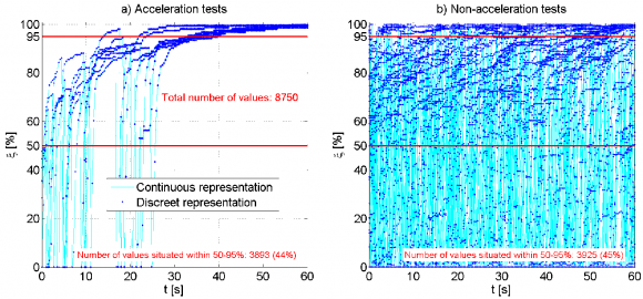
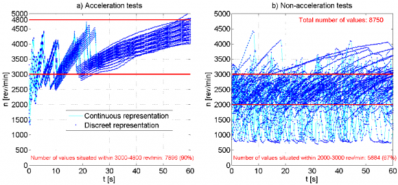
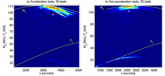
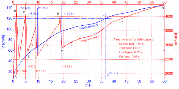
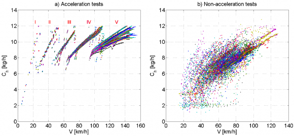
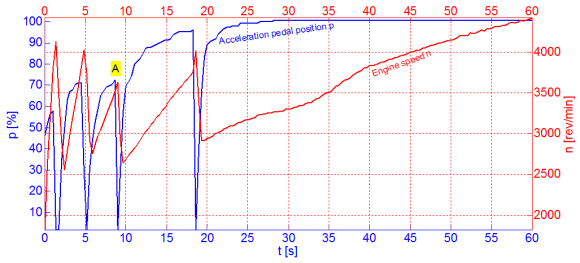
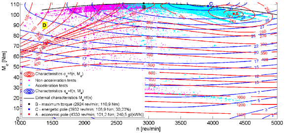
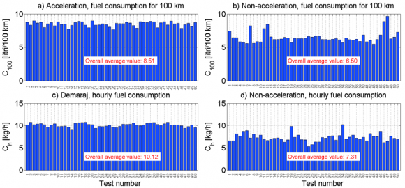
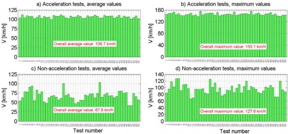
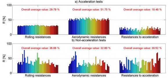
Theoretical study of the acceleration process is aiming to determine the calculus methodology for time and covered space by the vehicle until reaching the speed of 100 km/h; with these parameters, acceleration performances of various similar cars may be compared. [1; 3] Experimental study of acceleration allows the setting of performances in certain movement and driving conditions; thus the dynamic performances and real efficiency performances may be set. [2] In the paper herein a comparative study of acceleration is performed. The tests were carried out with a Logan Laureate vehicle that is equipped with an on-board computer. To this purpose 50 acceleration tests were selected and an additional 50 normal tests which are further on called non-acceleration tests. These later test describe a normal regular vehicle movement; speed variation character for the two cases is seen in figure 1, where also the maximum values overhaul are being presented. We have to underline that in classical, theoretical study, the vehicle's acceleration is being studied having the engine performing on its exterior characteristic, in full throttle in order to estimate maximum performances [1; 3]. In practical situations, the engine operates in partial loads [2]. Indeed, as we can see from figure 2a, the engine operates in 44% of situations at level or high loads and within 50-95% (different from full loads) approximately equal as the non-acceleration tests from figure 2b. As we can see from figure 2, engine load is appreciated by the throttle's angular position ?, as a percentage compared to its maximum opening position. In the literature engine load is also appreciated through the intake air pressure p a . Highlighting ranges where most experimental data are concentrated may also be observed in the parameters' bivariable dependence graph. To this purpose an example is being presented in figure 4, where the dependence from the engine speed and its torque is presented; the graphs also gives the external characteristic of the engine (B representing maximum torque) with its power P e and torque M e . As we can see from figure 4a, a great majority of torque values in the case of acceleration are found in the right side of maximum torque (in the area of high power output, area A). In exchange in the case of non-acceleration (regular movement), most values for the engine torque are in the left side of maximum torque (at lower power outputs). The graphs from figure 1a and 3a also highlight the fact that in the case of an electronically controlled vehicle it is difficult to notice the moments of time where gears are shifted if the vehicle's speed is targeted (figure 1a), but we need to analyze the engine's speed (figure 3a) The main cause is of course the rapidity with which the gears are shifted, without double clutching, with almost instantaneous shifting from one speed to another; the mentioned aspect is also revealed in figure 5 The two targeted forms of movement also have other particularities as we can see from figure 6 where engine hourly fuel consumption is presented C h . As we can see from figure 6a, in the case of acceleration we clearly can distinguish fuel consumptions through gears I-V, which is not the case for non-acceleration tests (figure 6b). The graphs also highlight the fact that as the vehicle speed V increases so does the fuel consumption. In order to better accentuate the nature of the process and their evolution tendencies a discreet representation of data was used. 8 presents engine torque M e depending on its speed n for various values of actual specific fuel consumption c e . In fact this represents the well known spatial static characteristic of engine c e =f(n, M e ), but transposed in 2D having izo-consumption curves where c e =const. (a so called complex characteristic). Based on this characteristic we get the classical economic pole, A dot on the graphic where c e =240,5 g/(kWh). Likewise, the graph also presents another spatial static engine characteristic that of ? e =f(n, M e ), also transposed into 2D having curves of constant engine efficiency ? e =const.; based on this the well known energetic pole is achieved, dot C where ? e =30.23%. The graph also presents the engine's external characteristic M e =f(n), on full load (for ?=100%), dot B being specific for maximum engine torque; we can see the energetic pole C is situated on the external characteristic. As we can see from figure 8, the experimental values specific for acceleration are closer to the economic pole A and to the energetic pole C than the case of the non-acceleration tests data; therefore, the engine is more efficient in case of acceleration. Higher fuel consumption values in the case of acceleration tests ensures higher vehicle speeds as we can see from figure 10, where average values and maximum values are presented for each test and overall. Comparing the upper graphs with the lower graphs we can see that in the case of the acceleration tests we achieved an average value for the vehicle speed which is 51.1% higher than the case of the nonacceleration test-runs and a maximum value which is 21.6% higher.