1. Introduction
haracterization of a given signal as noise like or tone like finds several applications in musicspeech classification [1,2,3], perceptual audio coding [4], Multi Band Excitation (MBE) model based perceptual coding of speech [5] and voice activity detection [6]. Within each category, the signals may be stationary/nonstationary/transient signal or gaussian/nongaussian. The Nongaussianity and/or nonstationary signal also occur when a radar signal is reflected by a fluctuating target or clutter [7] or when a communication signal passes through a fading wireless channel [8,9]. The fourth-order cumulant based kurtosis of the time signal was traditionally used for nongaussianity detection [10], Harmonic Retrieval from nongaussian processes [11], nonminimum phase system identification [12]. Recently the frequency dependent kurtosis defined in spectral domain was proposed and successfully used in bearing fault detection [13,14,15] and vibratory surveillance and diagnostics of rotating machines [16]. Spectral Kurtosis (SK) was originally introduced by Dwyer [17] where it was defined on the real part of the STFT filter bank output to overcome the deficiency of the power spectral density to detect and characterize the signal transients. Vrabie [18] justified the theoretical definition of SK and proposed an unbiased estimator of SK. Antoni [19,20] formulated SK differently by using Wold-Cramér decomposition with a theoretical basis for the SK estimation of non-stationary processes. He also practically used it for machine surveillance and diagnostics [16,21]. Other applications of spectral kurtosis reported in the literature include SNR estimation in speech signals [22], denoising [23] and subterranean termite detection [24].
In this paper, the important aspects of original spectral kurtosis theory is reviewed from fundamentals. The spectral kurtosis properties of both stationary and nonstationary signals as well as the stochastic mixtures are analytically obtained.
Extensive Monte Carlo simulations are carried out to support the theory reviewed and the spectral kurtosis of several processes at different signal-to-noise ratios (SNRs) is estimated. The results are in perfect match with the previous analytical findings.
The paper is organized section wise as follows. The mathematical basics of spectral kurtosis are introduced in the section II. The Test Signal Set comprising several popular signals are analytically described in section III. Short time fourier transform (STFT) for dynamically estimating the magnitude spectrum and the expression for estimation of SK from STFT is given in section IV. In Section V the details of Monte Carlo simulations of the Test Signal Set and the derived mixture processes, and the simulation results are presented. Finally the review summary and future work is given in Section VI.
2. II.
3. Spectral Kurtosis a) Background
Wold-Cramer's decomposition uniquely describes a non-stationary signal y(t) as the response of a causal linear system with time varying impulse response h(t, s) excited by a signal X(t) i.e.
4. ??(??
at time instant t-s. The frequency counterpart of eq.( 1) is given by
??(??) = ? ??(??, ð??"ð??") exp(??2??ð??"ð??"??) ????(ð??"ð??") ? ?? (2)where H(t, f) is the time varying transfer function of the system, which can be interpreted as the complex envelope of signal Y(t) at frequency f and dX(f ) is an ortho-normal spectral process associated with input driving process X(t). In many cases, H(t, f) is stochastic and can be represented with ??(??, ð??"ð??", ??) where ?? is a representative random parameter of filter's time varying transfer function. Let H(t, f) be conditioned to ?? i.e. the shape of H(t, f) depends on the outcome of the random variable ??. H(t, f, ??) can be assumed to be time stationary, stochastic and independent of the spectral process dX(f). Thus the signal X(t) is stationary in general but non-stationary for a particular outcome ??. Such a process was designated as conditionally nonstationary (CNS) process in [19]. It may be noted down that the simplest way to convert a nonstationary process to a CNS process is the time datum randomization. Any CNS process driven by a white process X(t) of order p ? 4 is likely to be leptokurtic i.e. its probability density function having tails flatter than those of its generating gaussian process and hence non-gaussian. In fact, this connectivity between the CNS and nongaussianity makes the kurtosis, originally defined on time processes to characterize the nongaussianity, a very useful in analyzing the nonstationary processes through kurtosis defined in spectral domain.
For the stationary white driving process X(t) of order p ? 2n, the spectral kurtosis of the nonstationary signal Y(t) is defined as the normalized fourth-order spectral cumulant [19] as
? ?? (ð??"ð??") = ?? 4?? (ð??"ð??") ?? 2?? (ð??"ð??") ? 2 = ??{|??(??, ð??"ð??")| 4 } ??{|??(??, ð??"ð??")| 2 } 2 (2 + ?? ?? ) ? 2 ? ?? ?? = ?? 4?? (ð??"ð??") (2 + ?? ?? ) ? 2 ? ?? ?? ð??"ð??" ? 0 (3)where the factor 2 in place of 3 as in usual definition of cumulants comes from the fact that dX(f) is a circular random variable, ?? 4?? (ð??"ð??") is the kurtosis of the (stochastic) frequency response of the time varying filter and ?? ?? is the time kurtosis of the input process.
If Y(t) is a purely stationary process, then ?? 4?? (ð??"ð??") is independent of frequency and is unity, then spectral kurtosis of Y(t) is given by
? ?? (ð??"ð??") = ?? ??(4)which is a constant and independent of the frequency.
In particular, the spectral kurtosis of a stationary gaussian process is zero (i.e. ?? ?? = 0).
5. b) Mixing Processes
Let Z(t) be the mixture of two processes (i) a non-stationary process Y(t) and (ii). a stationary additive noise N(t) .
??(??) = ??(??) + ??(??)(5)The spectral kurtosis of this mixture is given by [19] ?
?? (ð??"ð??") = ? ?? (ð??"ð??") [1 + ??(ð??"ð??")] 2 + ??(ð??"ð??") 2 ? ?? (ð??"ð??") [1 + ??(ð??"ð??")] 2 ð??"ð??" ? 0 (6)where ??(ð??"ð??") is the local Noise-to-Signal power ratio at the frequency f given by
??(ð??"ð??") = ?? 2?? (ð??"ð??") ?? 2?? (ð??"ð??")(7)If the mixing process N(t) is stationary (white or colored) gaussian process, then ? ?? (ð??"ð??") vanishes at all frequencies except at ð??"ð??" ? 0. Thus eq.( 6) becomes
? ?? (ð??"ð??") = ? ?? (ð??"ð??") [1 + ??(ð??"ð??")] 2 ð??"ð??" ? 0 (8)If the noise power is zero i.e. signal is clean, then ??(ð??"ð??") = 0 and hence
? ?? (ð??"ð??") = ? ?? (ð??"ð??") ð??"ð??" ? 0(9)When the process Y(t) is gaussian, eq.( 6) becomes
? ?? (ð??"ð??") = ??(ð??"ð??") 2 ? ?? (ð??"ð??") [1 + ??(ð??"ð??")] 2 ð??"ð??" ? 0 (10)where ??(ð??"ð??") is finite. If the noise power becomes larger and larger, ??(ð??"ð??") ? ?, the process Z(t) becomes purely the mixing noise process, the spectral kurtosis becomes
? ?? (ð??"ð??") = ? ?? (ð??"ð??") ð??"ð??" ? 0(11)III.
6. Test Signal Set
In what follows, some commonly found signals are considered for analytically computing the spectral kurtosis. The spectral kurtosis of some other signals not considered earlier is also obtained analytically.
7. a) Real Sinusoids
A real sinusoid of constant amplitude and constant frequency is given by
??(??) = ?? cos(2??ð??"ð??" 0 ?? + ??) (12)where ?? is a constant initial phase from ??(???, ??).
? ?? (ð??"ð??" 0 ) = ?? 4?? (ð??"ð??" 0 ) ?? 2?? (ð??"ð??" 0 ) ? 2 = ??{|??| 4 } ??{|??| 2 } 2 ? 2 = ?1(13)A real sinusoid of time varying amplitude and constant frequency is given by
??(??) = ??(??) cos(2??ð??"ð??" 0 ?? + ??)(14)If the amplitude decreases exponentially, the signal is called a damped sinusoid and is given by
??(??) = ?? ?? ????? cos(2??ð??"ð??" 0 ?? + ??) (15)where k is the damping (bandwidth) factor, ?? ????? is the decaying real envelope and ?? is the constant initial phase from ??(???, ??).
8. b) Random Amplitude Sinusoid
When a radar transmitted carrier signal is reflected by a fluctuating target, the carrier amplitude of the echo signal undergoes random fluctuations [7]. Similarly, a communication signal passing through a fading wireless channel, the amplitude of the signal at the receiver input undergoes random fluctuations [8,9]. In these cases, the time varying amplitude ??(??) in eq.( 14) can be represented by
??(??) = ?? ?? + ?? ?? (??) (16)where ?? ?? is the constant part and the random part ?? ?? (??) which is also called as the multiplicative noise. In case of deep fluctuations the constant part becomes zero and then ??(??) = ?? ?? (??). The spectral kurtosis of such a process is totally dependent on the probability density function of ?? ?? (??). In [25] the spectral kurtosis of such a random amplitude sinusoid was shown to be
? ?? (ð??"ð??") = ?? ?? ?? + 1 (17)where ?? ?? ?? is the coefficient of kurtosis or time kurtosis of the random amplitude. The coefficient of kurtosis ?? ?? ?? based on cumulants can be obtained from the following expressions [26,27].
?? 2 = ?? 2 ? ?? 1 2 ?? 4 = ?? 4 ? 4?? 1 ?? 3 + 6?? 1 2 ?? 2 ? 3?? 1 4 ?? 2 = ?? 2 ?? 4 = ?? 4 ? 3?? 2 2 = ?? 4 ? 3?? 2 2 ?? ?? ?? = ?? 4 ?? 2 = ?? 4 ?? 2 2 ? 3 (18)where ?? ?? are the k-th standard moments, ?? ?? are the kth central moments and ?? ?? are the cumulants. a) If the amplitude of the random sinusoid in eq.( 16) is totally random with a gaussian density function, then from eq.( 17) and eq.( 18), the spectral kurtosis is given by
? ?? (ð??"ð??") = ?? ?? ?? + 1 = 3?? 4 (?? 2 ) 2 ? 3 + 1 = 1 (19)b) If the amplitude of varies uniformly in the range (a, b), then the spectral kurtosis from eq.( 17) and eq.( 18) is given by
? ?? (ð??"ð??") = (?? ? ??) 4 80 ? ? (?? ? ??) 2 12 ? ? 2 ? 3 + 1 = 144 80 = ?0.2 (20)c) For a rayleigh distributed random amplitude, the standard moments are given by
?? 2?? = 2 ?? ?? 2?? ??! ?? = 1,2Then from eq.( 17) and eq.( 18), the spectral kurtosis can be obtained as
? ?? (ð??"ð??") = 0 (21)9. c) Harmonic and Inharmonic Sinusoids
A harmonic sinusoid comprises a sine wave of fundamental frequency ð??"ð??" 0 and its finite number of harmonics ð??"ð??" ?? = ??ð??"ð??" 0 as denoted by
??(??) = ? ?? ?? cos(2????ð??"ð??" 0 ?? + ??) ???1 ?? =0 (22)where M is the number of harmonics. The amplitudes of the harmonics decay at different rates depending on the instrument or the note played. A typical profile of the harmonic amplitudes is given by ?? ?? = 1/??. If the frequencies are independent and no harmonic relation among them i.e. ð??"ð??" ?? ? ??ð??"ð??" 0 , then the sinusoids are called inharmonic sinusoids. Both harmonic and inharmonic sinusoids appear frequently in music produced by several instruments.
10. d) Additive Gaussian Noise
Additive White Gaussian Noise (AWGN) signal is a noise commonly found in communication channel which adds to the transmitted signal. The spectrum of this signal is flat with a constant one-sided power spectral density ? within the channel bandwidth.
If power spectral density of the noise within the channel bandwidth is function of frequency, then the Similarly the spectral kurtosis for other density functions can be obtained. The focus of this paper is not to derive such expressions, but to show that ? ?? (ð??"ð??") is a positive constant depending on the probability density function. However for some more density functions, the simulations are carried out as described in the section V.
noise is called colored noise and is characterized by ?(f).
11. e) Modulated Signals
An amplitude modulated signal with a carrier frequency f c modulated by a sine wave of a low frequency f m and is given by
??(??) = ?? ?? (1 + ?? ?? ??????(t) cos(2??ð??"ð??" ?? ?? + ??) (23??)where ?? ?? is the amplitude of the carrier and ?? ?? is the modulation index, ??????(??) is the low frequency message signal. The Double Side Band (DSB) signal, the Lower Side Band (LSB) signal and the Upper Side Band (USB) signal can be formed by appropriate processing the AM signal.
The Frequency Modulated (FM) signal can be obtained as
??(??) = ?? ?? cos ?2??ð??"ð??" ?? ?? + 2?? ?? ð??"ð??" ? ??????(??)???? ?? 0 ? (23??) f) Chirp SignalA chirp signal is a frequency modulated signal in which the frequency of the carrier is linearly or hyperbolically varied. This kind of chirp signal is extensively used in pulse radars for achieving higher range resolution using a longer transmitted pulse, which is otherwise possible with a shorter transmitted pulse [14]. A phase modulated signal is given by
??(??) = ?? cos ??(??) = ?? cos 2??ð??"ð??"(??)?? (24)where ??(??) is the time-varying phase of the carrier. The frequency profile f(t) can be linear, quadratic or logarithmic.
In a linear chirp signal, the carrier frequency f is varied as ð??"ð??" ?? + ????, where ?=df/dt is the chirp rate. Then time-varying phase of the carrier is given by
??(??) = 2?? ? ð??"ð??"(??)???? ?? 0 = 2?? ? (ð??"ð??" ?? + ???? )???? ?? 0 = 2?? ? ð??"ð??" ?? ?? + 1 2 ???? 2 ? (25)Substituting eq.( 23) in eq.( 22), we get
??(??) = ?? cos 2?? ? ð??"ð??" ?? ?? + 1 2 ???? 2 ? (26)If the start frequency at ?? = 0 is f c and the end frequency at ?? = ?? 1 is f 1 , then the chirp rate is given by ?
= (f 1 -f 0 )/t 1 .In a quadratic chirp signal, the instantaneous frequency is given by
ð??"ð??"(??) = ð??"ð??" ?? + ???? 2 (27)where ?? = (ð??"ð??" 1 ? ð??"ð??" 0 )/?? 1 2 .
In a logarithmic chirp signal, the instantaneous frequency is given by
ð??"ð??"(??) = ð??"ð??" ?? ?? ?? 1 (28)where ?? = (ð??"ð??" 1 /ð??"ð??" 0 ) 1/?? 1 .
IV.
12. STFT Based Spectral Kurtosis Estimation
In this section a means of estimating the spectral kurtosis from the short time fourier transform (STFT) is presented. Here the input signal y(n) is divided into overlapping or non overlapping frames each of size N, multiplied by a window function w(k) like a hamming window of same size and analyzed by using the Fourier Transform. A matrix popularly known as a spectrogram is formed by arranging STFT coefficients as columns as given by
??(??, ??) = 1 ???? ?? ?? ?? ?? (?? + ????) ??(??)?? ??? 2?? ???? ?? ???1 ??=0 ? 2 0 ? ?? ? ?? ? 1, 0 ? ?? ? ?? ? 1 (29)where k is the frequency index, l is the time frame index, M is the hop size, K is the total number of frequency bins of one-sided STFT and L is the total number of frames contained in the signal. An un-biased estimator of the spectral kurtosis is proposed in [19] based on L realizations of K-sample signal. The discrete fourier transform (DFT) on a Ksample signal computes the signal spectrum at Knumber of discrete frequencies. If the L number of nonoverlapping frames used in the STFT analysis are considered as L number of the independent stochastic signal realizations, the spectral kurtosis ? ?? (?? 0 ) at the frequency index ?? 0 can be computed from the ?? 0 -th row of the spectrogram matrix ??(?? 0 , . )The spectral kurtosis at all frequency indices 0 ? ?? ? ?? ? 1 is given by
? ?? (??) = ?? ?? ? 1 ? (L + 1) ? ? |??(??, ??)| 4 ???1 ??=0 {? |??(??, ??)| 2 ???1 ??=0 } 2 ? 2? 0 ? ?? ? ?? ? 1(30)13. Simulations and Results
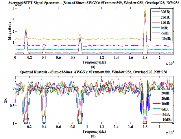
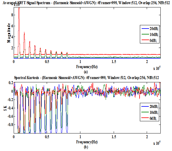
The following signals are simulated using eq.( 12), eq.( 14), eq.( 15) and eq.( 20) through eq.( 28). A composite signal if formed by summing four sinusoids of frequencies 1800Hz, 4000Hz, 9000Hz and 18000Hz with respective amplitudes: 1.0, 0.25, 0.7 and 2.0 is formed. An additive white gaussian noise (AWGN) is added to the composite signal to form the first mixture process. Thus the mixture comprises a total five signals: four constant amplitude sinusoids and gaussian noise. The variance of AWGN is adjusted so as to obtain signal-to-noise ratios of 30dB, 20dB, 10dB, 0dB, -5dB and -10dB.
The mixture signal is generated for a duration of 1.1610 seconds. STFT is computed for frames or window size of 256 samples with 50% (i.e. 128 samples) overlap. Each frame is multiplied by a hamming window of 256 samples and a 256-point FFT is computed thus giving a spectrogram matrix of size 256 × 399 ??(??, ??) ; 0 ? ?? ? 255, 0 ? ?? ? 398 each of 256 frequency bins of spectrogram matrix is averaged over 399 frames to obtain a mean STFT spectrum ?? ?? (??) = ???(??, . )?; 0 ? ?? ? 255 which is called here as Averaged STFT Spectrum. Fig. 1a gives the Averaged STFT Spectrum of Mixture-1 for different SNRs. Four peaks of different amplitudes observed in the spectrum correspond to four sine waves in the mixture. The low amplitude second peak is submerged in the noise floor at low SNRs below 0dB. As the SNR decreases, the noise floor also increases. The spectral kurtosis ? ?? (??); 0 ? ?? ? 255 is also computed from the spectrogram matrix using eq.(28) as explained in section IV. It may be noted that ? ?? (0) is to be ignored, as the kurtosis is not defined at ð??"ð??" = 0. The Fig. 1b gives the spectral kurtosis (SK) of Mixture-1 for different SNRs.
The spectral kurtosis has four negative peaks corresponding to four sinusoids. For higher SNR (30dB) the peaks have a value of -1 irrespective of the sinusoid amplitudes. As the SNR decreases, the peaks values increase from -1 towards zero. Local SNR computed at peak locations vary depending upon the amplitude of the sinusoid. Here it is maximum at 18000Hz and minimum at 4000Hz. It may be noted down that the SNR referred in the legend of the figures1(a) and (b) is the global SNR, which is computed based on the aggregate of all sinusoids. For global SNRs below 0dB, where the AWGN power dominates the aggregate power of all sinusoids, the mixture becomes more and more gaussian, the spectral kurtosis tends to zero, relatively faster at 4000Hz where the local SNR is minimum. b) Mixture-2
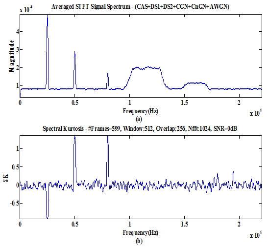
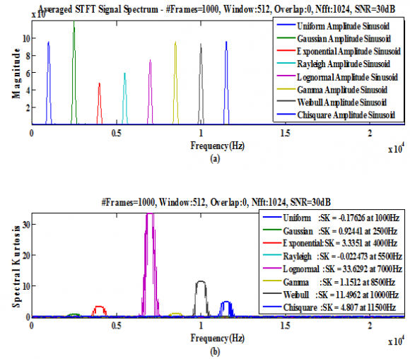
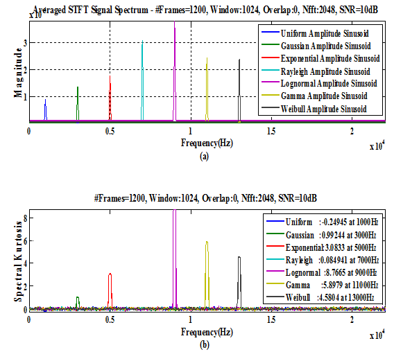
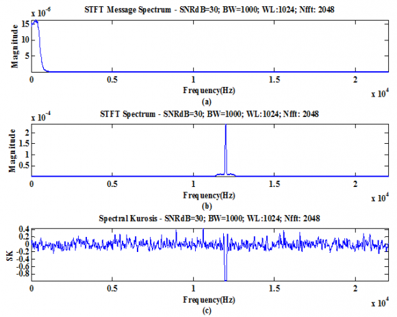
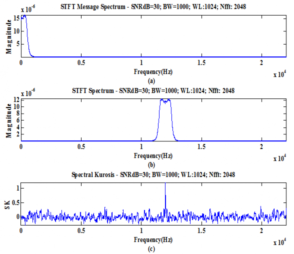
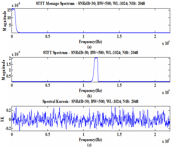
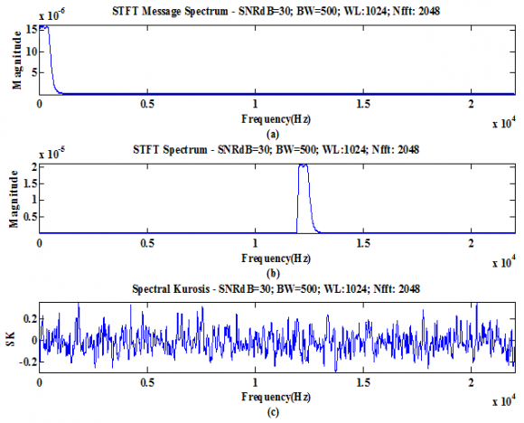
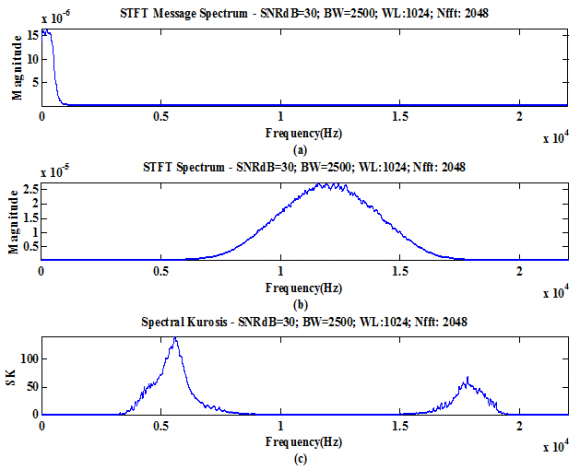
The second Mixture process comprises six components: constant amplitude sinusoid(CAS), two damped sinusoids(DS1 and DS2) with different damping factors, colored gaussian noise(CGN), colored uniform(i.e. nongaussian) noise(CnGN) and AWGN. Global SNR is computed with respect to AWGN considering the other five components as composite signal. The CGN is obtained by passing white gaussian noise through a 6-order butterworth band pass filter having passband between 10KHz and 13KHz. The CnGN obtained by passing white uniform noise through a 6-order butterworth band pass filter having passband edges at 15KHz and 17KHz. 20). The SK of the second sinusoid at 2500Hz is +1.0, corresponding to gaussian distributed amplitude variations (see eq. 19). The SK of fourth sinusoid at 5500Hz is 0.0, corresponding to rayleigh distributed amplitude variations (see eq.21). The fourth Mixture is basically a harmonic sinusoid with a fundamental at 800Hz and having 10 harmonics contaminated by an AWGN. The amplitude of n-th harmonic is 1/n, but this amplitude remains constant with time. The STFT spectrum of this mixture is shown in Figure 5(a) for SNRs of 20dB, 10dB and 0dB. The ten negative peaks in SK plot of Figure 5(b) correspond to seven sinusoids. Please note that each peak is -1 irrespective of the harmonic number for higher SNRs. As SNR decreases, the negative peaks move from -1 towards zero. The SK of AM signal is -1.0 since the carrier is strong due to low modulation index and resembles a constant amplitude at carrier frequency of 12KHz.. The SK of DSB is positive at carrier frequency of 12KHz showing its nonstationary nature. The SK of the next two mixtures LSB and USB is over the signal bandwidth. However, at the band edges, the SK takes exceptionally large values.
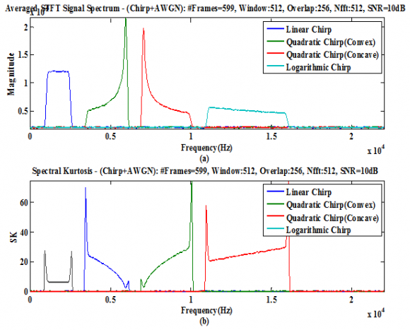
14. f) Mixture-6
The sixth Mixture is made up of different chirp signals: linear, quadratic and logarithmic chirps generated using the eq.( 24) through eq.( 28). Each chirp is shown in different colors in Fig 11. The STFT spectrum of this mixture is shown in Figure 11(a
15. Conclusions and Future Work
The cumulant based spectral kurtosis defined in frequency domain originally proposed for bearing fault detection and monitoring of electrical machines, is a promising tool for analyzing nonstationary signals. It complements the traditional power spectrum based on second order statistics. In this paper, the theory of spectral kurtosis is briefly reviewed from the fundamentals. The properties of spectral kurtosis of popular stationary signals, nonstationary signals and mixed processes are analytically given.
Extensive Monte Carlo simulations were carried out to support the theory. The spectral kurtosis of the simulated stationary, nonstationay and mixed processes at different signal-tonoise ratios (SNRs) is estimated and the results are in good match with the previous analytical findings. The review highlights the usage of spectral kurtosis for other areas of signal processing like communications and radar signal processing. Future work could be (i). Obtaining closed-form expressions for spectral kurtosis of communication and radar signals (analog or digital modulated) (ii). classification of communication signals using spectral kurtosis at different SNRs.(iii). radar signal classification using spectral kurtosis.