dvances in computation and improved mapping techniques allow increasingly precise assessment of the attributes mapped. Examples are the data interpolation methods used to determine spatial representation models. The use of GIS has made it much simpler to visualize and manipulate field data as well as to carry out spatial analyses and detect similar patterns, to help understand natural phenomena. Such systems can be applied to manage river basins, where all the information regarding hydrological variables, topo-bathymetric sections, land use and plant cover, among other aspects, enables the use of mathematical models to simulate the river behavior.

Modeling the hydrodynamic conditions of a watercourse's flow allows identification of areas subject to flooding and establishment of the flood levels for the risks chosen [1]. In this respect, to help update the results indicated by [2] obtained from the Macacu Project, in this study we attempted to develop new hydraulic simulations from data obtained in a new topographic survey carried out by the Rio de Janeiro State Environmental Secretariat [3] in the basin of the Guapi-Açu River, a tributary of the Macacu River, located in the eastern part of the Guanabara Bay Basin, in Rio de Janeiro state, Brazil. For this purpose, information from the project's GIS was integrated with the HEC-GeoRAS interface to feed the computational model in the HEC-RAS hydrodynamic modeling program in one dimension, and the results were compared with those produced by a two-dimensional IBER model, simulating unsteady flood wave regimes referring to return periods of 2, 10, 20 and 50 years.

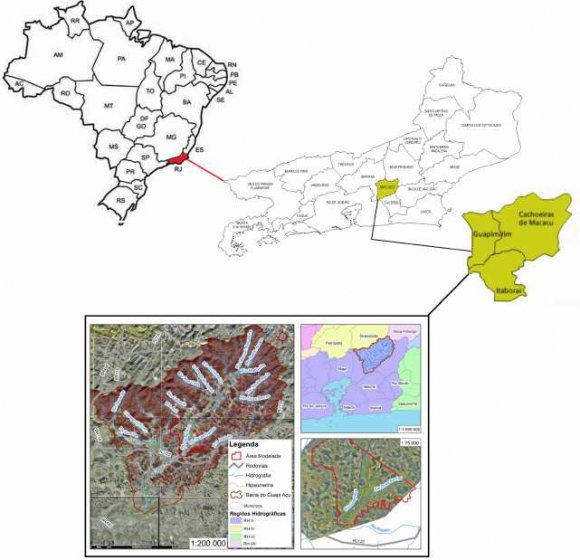
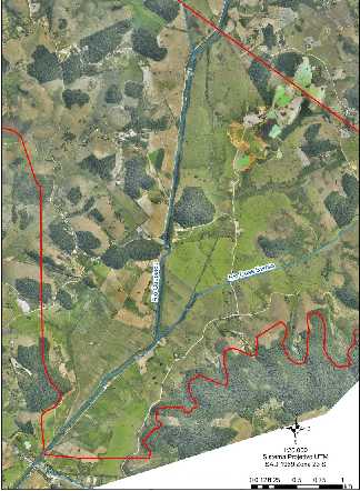
The Guapi-Açu River Basin is located in the eastern part of the Guanabara Bay Basin, Rio de Janeiro state, Brazil, as shown in Figure 1. This river basin is very important regarding water availability in the region, since it is responsible for supplying water to the region through the Imunana-Laranjal supply system [2]. The basin drains an area of approximately 560 km², with its main river, the Guapi-Açu, which flows into the Macacu River, together forming the Guapi-Macacu Basin. The basin covers parts of three municipalities, Cachoeira de Macacu, Itaborai and Guapimirim.

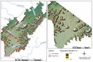
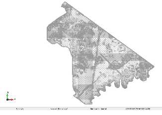
Hydraulic modeling requires a high level of topographic precision. In this study we used aerial photographs on a 1:8,000 scale supported by field survey data, provided by [3]. The area covered by these data starts at about 1 km from the bridge along highway RJ-122 crossing the Guapi-Açu River and reaches in a line of about 15 km in the upstream direction. However, due to the large computational effort for each simulation (average time more than 6 hours), we decided to reduce the area to be modeled to the segment between the bridge and 6 km in the upstream direction, as shown in Figure 1 inside the red outline. We divided the methodology adopted into three steps: According to [4], the computational instruments used in geoprocessing are called geographic information systems (GISs). Their purpose is to facilitate analysis by integrating data from different sources, creating a database containing georeferenced data. Based on this concept, we structured a GIS for the Guapi-Açu Basin from cartographic, planimetric and altimetric bases, on a scale of 1:8,000, with vertical distance between contour curves of 1 m. The software used was ArcGIS 10.1 from the Environmental Systems Research Institute (ESRI). The second step for structuring the GIS was to create a digital terrain model (DTM). This model can be understood as a synthetic surface representing the spatial distribution of the altimetry of a land area, which has continuous variation in the area of interest. According to [5], geomorphological and hydrological consistency is attained when the raster of the DTM faithfully represents the characteristics of the terrain, such as the division lines of river basins, channels and concave and convex relief forms, and assures convergence of the surface flow to the drainage network mapped. Further according to him, the interpolation tool to generate the best DTM in terms of hydrological consistency is Topogrid. The correction of the relief by this model is carried out by a combination of local and global interpolation methods [6]. This combination allows sudden changes in slope in the drainage areas and dividing lines to be adjusted, generating a characteristic connected drainage structure defined by the erosive force of the water, a result also corroborated by [7]. The interpolation by Topogrid for the study area is presented in Figure 1 and further expanded in Figure 2. The left part shows the entire region where the topographical survey was carried out by [3] while the right part shows the area considered in the simulations. At the end of the interpolation, the spatial resolution was 2 meters, i.e., the side of each pixel was 2 meters, meaning each cell of the DTM, measuring 4 m², had a single altimetric value. In structuring the DTM we used all the data from the survey, to minimize possible interpolation errors. The highest and lowest altitudes resulting from the DTM were 222.5 meters and 0.47 m.

The available information on the Guapi-Açu Basin comes from the Macacu Project developed by [2]. This project was a pioneering effort, for the purpose of constructing a dam called Guapi-Açu Jusante as a solution to meet water demand of the region, since the water basin is responsible for supplying water to about 2.5 million people. According to [8], the rainfall modeled in a hydrographic project is an idealized event associated with a return time (RT). In the present study, the RTs chosen were 2, 10, 20 and 50 years. To estimate the rainfall duration, we assumed it is equal to the concentration time in the basin studied, calculated by the formula proposed by Ventura [9], expressed by:

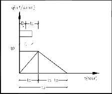
(1) Where tc is the concentration time, in minutes; A is the drainage area, in km²; L is the length of the thalweg, in km, and Î?"H is the difference in height between the highest point of the thalweg and the outflow point, in m. After making the substitutions, considering the drainage area of 291.5 km², thalweg length of 26.5 km and hydraulic head of 1.085 meters, this equation produced a concentration time of 10.68 hours. The flow volume was estimated by the triangular unit hydrograph (TUH) method, proposed by the former United States Soil Conservation Service (SCS), now called the National Resources Conservation Service (NRCS). According to [8], this is one of the simplest and most widely used methods to estimate the surface runoff volume. In the TUH, the triangle's base represents the duration of the surface runoff (tb), the height represents peak flow (qp) and the area is the surface runoff volume (V), as indicated in Figure 3. Therefore, the parameters that characterize it are:

Where tp is the peak time, in hours; ta is the ascension time, in hours; tb is the base duration time, in hours and D is the duration of the unit rainfall, in hours.

Substituting the surface runoff volume in the unit hydrograph equation ( 3) by the product of the basin area and an excess rainfall unit, and considering equation ( 6), yields the expression to calculate the peak flow of the hydrograph:

Where qp is the maximum flow for 1.0 mm of excess rainfall, in m3.s-1.mm.

The rainfall assumed in the project was taken from [10], expressed by: (7) Where I is the rainfall intensity, in mm/h; RT is the return time, in years, and t is the rainfall duration, in minutes.

To transform the rainfall into a uniform precipitation throughout the basin, we adopted the formulation proposed by [11], expressed by: (8) Where P is the distributed rainfall, in mm; Po is the rainfall, calculated from the equation ( 7), in mm; Ao is the basin area, in km², for which P equals Po. According to [11], it is usual to adopt Ao ? 25 km².

After defining the distributed rainfall, it is necessary to characterize the soil infiltration capacity, which is affected not only by the soil type, but also by the plant cover and type of land occupation and use in the basin in question. This parameter is defined by: (9) Where S is the potential retention of the soil, in mm and CN is the curve number, a function of the type of occupation. For the present study, we used a curve number equal to 50.

To construct the hydrograph it is necessary to define the effective rainfall (Pe), expressed in mm, which represents the portion of the rainfall that generates surface runoff. It is a function of the distributed rainfall and the soil retention potential and is defined as: Various authors and organizations have presented computer programs to solve equations describing non-uniform flows in watercourses, both in steady and varied regimes. In this study we adopted the HEC-RAS model and the IBER model.

The HEC-RAS model and its extension to the GIS environment are free programs that can be found at the site www.hec.usace.army.mil/software/, produced by the US Army Corps of Engineers at the Hydrologic Engineering Center. It is a computational model to analyze the flow in watercourses and is currently available in version 4.1.

Over the years the program's capacity has been expanded so that it now can represent rivers with a combination of regimes, compound sections, bridges, sluices, culverts etc. The HEC-GeoRAS extension employed here allows the introduction of data automatically, as proposed by [12], and allows the identification of areas subject to flooding, besides establishing flood levels for chosen risks [1]. Its main limitation is that it is a one-dimensional model that works with cross-sections of the river of interest, so it does not produce good results for the unsteady flow regime. The arrangement of the cross-sections and the spacing between them, are depicted in Figure 4. We set out 36 cross-sections, with average length of 2,000 meters and average spacing of 200 meters. From Figure 5, it can be seen that the predominant land use is agriculture, with pasture along the river banks, with some areas of remaining forest and secondary vegetation. Table 1 reports the breakdown of land use and the respective Manning coefficients.

Table 1 : Land use and respective Manning roughness coefficients, as adapted from [13] ii. IBER Model The IBER model is also free and was developed by Universidad de A Coruña (UDC), Universitat Politècnica de Catalunya (UPC) and Centro Internacional de Métodos Numéricos en Ingeniería (CIMNE).

It can be downloaded from http://iberaula.es/web/index.php. The IBER is a numerical simulation model of free flow and environmental processes in fluvial hydraulics, and can be applied to model river hydrodynamics, dam failures, flood-prone zones, sediment transport and tidal flows in estuaries.

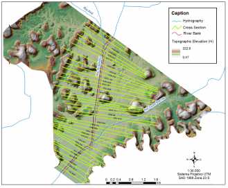
The first step of the hydrodynamic modeling was to introduce the DTM in the model, with all the information on relief maintained (georeferenced data). This involved creating a triangular mesh with minimum sides of 2 meters and maximum of 100 meters, in the format of the DTM as shown in Figure 6. After introducing the DTM, it was necessary to indicate in the mesh created at the entry position of the hydrograph, i.e., the upstream part of the Guapi-Açu River, as well as the exit from the hydrograph. As can be seen in Figure 6, the geometry is similar to that presented in the right side of Figure 2. The other condition added to the model was the inclusion of the Manning roughness coefficients, according to the values indicated in Table 1 for each type of land use.

By applying the formulas, it was possible to define the hydrographs. The peak flows with return times of 2, 10, 20 and 50 years are, respectively, 11.5 m³.s-1, 78.0 m³.s-1, 136 m³.s-1 and 256 m³.s-1, in all cases happening about 15 hours after the start of rainfall. The total response time of the basin to rainfall is about 30 hours. These hydrographs were used to establish the boundary conditions in the simulations.

For evaluation of the results produced by the one-and two-dimensional hydrodynamic models, in the next sections we present the input and output hydrograph of the river segment modeled, assuming a buffering effect of the natural channel and adjacent overflow areas, as well as maps showing flooded areas, to enable comparison of one model against the other.

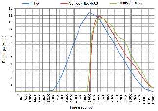
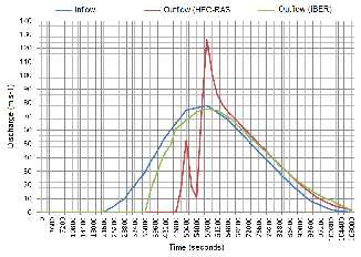
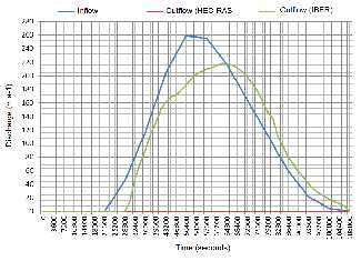
The results of simulating the flood wave with return time of 2 years are presented in Figure 7. The blue line is the input in the models for RT of 2 years while the red line is the output of the HEC-RAS simulation and the green line is the output of the IBER Both models present a buffer effect from the inflow peak, which was expected. The HEC-RAS presents a less pronounced buffer effect than the IBER, but the outflow volume presented by the IBER is greater than that of the HEC-RAS. Furthermore, the IBER output presents small elevations, in the form of peaks, while the 1D model does not show these peaks.

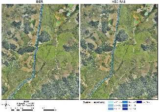
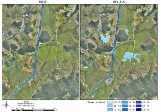
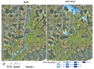
The maps in Figure 8 show the areas subject to flooding with a return time of 2 years (IBER on the left and HEC-RAS on the right). The increase in the peak outflow in relation to the inflow in the HEC-RAS simulation can be explained by the fact that at some points along the river the channel cannot hold the flow for a RT of 10 years. However, in the recession portion of the hydrograph, both the 1D and 2D models present similar aspects.

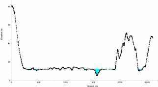
Figure 10 presents the inundated areas by passage of the flood wave for the 10-year RT (IBER on the left and HEC-RAS on the right). The maximum water level in the two models is 0.0 to 8.0 meters above ground level. The highest water levels are in the river's natural channel. As can be seen in Figure 11, the marginal areas of the main channel flood as soon as the water level in the section reaches the highest land elevation, i.e., in the main channel delimited by the margins (red points), and when the water level rises above the land adjacent to the channel, these are also considered areas reached by the flooding, due to the fact the HECRAS is a 1D model. The arrow indicates a place where there is no connection with the main channel, but the program considers it to be flooded even though the channel and the valley are separated by a ridge and are 1 km apart. When this information is taken to the GIS environment through the HEC-GeoRAS extension, these patterns are incorporated and appear on the map as flooded areas.

iii. 20-year return time

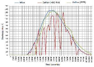
The results of simulating the flood wave with return time of 20 years are presented in Figure 12. The peak inflow is 136.4 m³.s-1 against peak outflows of 130.8 m³.s-1 for the HEC-RAS and 133.1 m³.s-1 for the IBER. It can be seen that the hydrograph generated by the HEC-RAS simulation presents large peaks and troughs. According to [14], in an unstable numerical model, certain types of numerical error are magnified as the solution starts to oscillate, or the errors become so large that the calculations cannot continue. That fact here is due to the large flood plains adjacent to the channel, a feature that destabilizes the mathematical model, producing an incorrect output hydrograph. This instability occurred for the flows equal to or greater than that of the 20-year RT, preventing the simulations from presenting reliable results, or causing the model not to present any results at all.

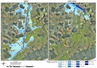
Figure 13: presents the flood map for a RT of 20 years. The difference between the two models is clear. In the IBER simulation the adjacent flooded area is much smaller than that produced by the HEC-RAS. The IBER simulation can be considered more coherent with the ground levels, with flooding in the lowest areas, while the HEC-RAS model, due to the numerical instability, presented erroneous results, because all theflow remained upstream of the segment studied, inundating adjacent areas. In the simulation of a 50-year RT, the buffer effect occurring in the natural channel was significant, due to the fact the alluvial plains are reached by the flood wave, buffering the flow in the main channel.

The map with the flooded areas for the RT of 50 years is presented in Figure 15, which depicts large areas reached by the flood wave, located in the lowestlying areas and in the meanders of the affluent rivers of the Guapi-Açu River and in irrigation canals.

Once again, the HEC-RAS model was unstable, and the result for flooded areas is not coherent. The overflow of the river channel occurred in the upstream part, as if all the flow would accumulate in the marginal areas, without any flow in the main channel. The IBER model presented large areas subject to flooding, but in these areas the water level was not greater than 2.0 meters above land height, while in the main channel the water level reached 10 meters above the land.

V.

The HEC-RAS is an intuitive and easily manipulated program with user-friendly interface that presents reliable results for simulation of steady flow regimes, with low computational cost and time. Modeling with this program requires less input data than 2D models, without the need for great details like those from DTMs and other boundary conditions.

Based on the results of this study, we suggest using the HEC-RAS in regions where the main watercourse is well contained by the surrounding terrain, without large floodplains and confluences with other rivers. Nevertheless, it is still possible to generate good flood maps using this one-dimensional model as long as attention is paid to cases where calculation instability occurs in the unsteady regime. For the river segments similar to that studied here, the HEC-RAS model is recommended for passage of the flood wave with RT of 2 years, because it required less simulation time (only minutes) than the IBER model, which took hours, and the results of the two models converged, both for the outflow hydrograph and map of flooded areas.

However, to describe many natural phenomena, such as rivers with extensive floodplains, the confluence of rivers and wide and irregular channels, one-dimensional model can no longer be considered adequate.

The two-dimensional model presented results more compatible with what would really occur, but models like the IBER require data that are more attuned to the natural terrain conditions for the simulation to attain a reasonable degree of accuracy. This requires more precise topographical studies, making this modeling more expensive. Another relevant fact is that two-dimensional models require much more computational resources and time to produce satisfactory results. In the particular case of the IBER, although it has user-friendly interface, it is still very recent and is being improved, so it still presents some problems in inserting boundary conditions.

In summary, the two-dimensional model presented more coherent results for flows that overflowed the channel of the Guapi-Açu River, including presenting buffer for the return times of 50 years. Each model has its own peculiarities, and the user must judge which tool is best depending on the case. Both have good potential for use by planners when integrated with a GIS.