1. INTRODUCTION
n linear quadratic previewed control, tracking performance by the feedforward control proportional to an exogenous input is well known [1][2][3][4][5]. The state space model in these problems incorporates a strictly proper system. However, models that employ sensors to measure exogenous inputs are sometimes biproper. A classical example is a small aircraft regulation in cruise condition wherein the normal acceleration is regulated for a smooth ride quality in the presence of gust inputs. For such systems, previewed control for biproper system is required. In this paper, the procedure for strictly proper system in Ref. 1 is extended and a modified Riccati matrix differential equation for biproper system is studied further.
There is substantial progress in gust alleviation [6,7] and in structural control problems with accelerometers [8] that are biproper systems. Yet, especially in gust alleviation, investments for forwardlooking sensor have been made to measure the presence of gust ahead of a flight path [9]. We are required to use the previewed measurements and restore the performance in the time windows of gust using a feedforward control law. Therefore, linear quadratic previewed (LQP) control for biproper systems is considered. In normal acceleration regulation, the inner loop controller is assumed fixed. Thus, the feedforward actions linear to the measurements of exogenous inputs are considered in simulation.
It is possible to convert a biproper system into a strictly proper system and develop a LQP control within Author : Professor, Department of Aerospace Engineering, Jain University Global Campus Jakkasandra Post, Kanakapura Taluk Bangalore Rural, India, 562 112. Email: [email protected] the framework of strictly proper system. To this end, consider a scalar differential equation with respect to time, [10,11].
) ( ) ( ) ( ) ( ) ( ) ( t duIn Section 2, modified RDE and its symmetric matrices are presented. Section 3 provides stability and optimality conditions to solve the RDE. In Section 4, a scalar example is used to compare the tracking performance of biproper and strictly proper systems. Conclusions are presented in Section 5.
2. MAIN RESULTS
In deriving an optimal control law
p t is,1 1 2 2 ( ), ( ) ( ), ( ) ( ), ( ) ( ), ( ) ( ), ( )3. H e t Qe t u t Ru t Ax t p t Bu t p t Ew t p t (5)
Following the necessary conditions for optimality,
4. & ( ) ( ) ( )
5. H H p t u t x t
We have the control law as a function of the costate vector,
1 ( ) [ ( ) ] u R DQD Bp DQCx DQ z Fw (6) ( ) p A p CQDu C QCx C Q z Fw (7)Here (.) refers the transpose of the vector or matrix (.) . For brevity, the time variable in the arguments is suppressed. Since 0 Q (positive semidefinite) and 0 R (positive definite), the sufficient condition,
2 2 ?0, H R R D QD u for a minimum ( )u t is met. Rewriting Eqn.( 7)
1 1 ?( ) ( ) [ ] p A p WR W C QC x C Q WR D Q z Fw ,(8)the matrices W C QD and
( ) { [ ]}, [ , ] u t R Kx B g D Q z Fw t t T . (10)The state feedback gain and the closed loop system matrix are defined as below,
K B K W (11) 1 1 ??[ ]. c x A x BR B g Ew BR D Q z Fw (12)Note that in the stability matrix A is stable. Consider the time derivative of ( ) p t in Eqn. (9),
1 1 1 ?[ ] ? [ ] p K KA KBR B K x KBR B g g KEw KBR D Q z Fw (13)Equating the coefficients of like terms in Eqn.( 7) and (13), the RDE and g -equation for tracking performance are,
1 1 ?K KA AK KBR BK WR W CQC (14) 1 [( ) )] [ ] c g A g KB W R D C Q z Fw KEw (15)The boundary conditions for the forward integration are known to be g(T) = 0 and 0 0 ( ) K t K . For finite duration optimal control problem in time 0
[ , ] t T , the transversality conditions [1], lead to the following end conditions,
1 1 ( ) [ ] K T S C QC WR W (16) 1 1 ( ) [ ][ ( ) ( )] g T S C Q WR D Q z T Fw T (17) 1 ? I WR B and W C QD Note that when ( ) ( ) Fw t z t , the reference signal ( )z t is previewed. The optimal control law in Eqn.(10) minimizing J can be stated as follows:
Control Law: Given the linear time invariant system Where ( ) u t is unconstrained, T is specified, R is positive definite, and Q and Q are positive semidefinite. The optimal control exists, is unique, and is given by
( ) ( ) ( ) ( ) x t* 1 0 ( ) { [ ]}, [ , ] u t R Kx B g D Q z Fw t t T .The n by n real, symmetric and positive definite matrix K in K B K W is the solution of the Riccati type matrix differential equation in Eqn. (14) with boundary condition in Eqn. (16). The vector ( ) g t (with n components) is the solution to the linear vector differential equation in Eqn. (15) with the boundary condition in Eqn. (17). The optimal trajectory is the solution of the linear differential equation in Eqn. (12).
6. III. STABILITY AND OPTIMALITY CONDITIONS
Consider matrix ? and the sufficient condition ?0 H for local optimality, where
2 2 2 2 2 2 ?? H Q W x x u H W R H H u x u.
In cases where 0 D , a positive semidefinite ? is guaranteed by the virtue 0 Q and 0
7. R
. In biproper systems, however, it is necessary to select quadratic weights 0 Q and 0 R such that ? is positive semidefinite for a given non-zero W . To derive stability, consider the algebraic Riccati equation,
c c KA A K KBR B K WR W C QC Q .Clearly, stability is guaranteed if ?0 Q . Therefore, given ?0 R and 0
8. Q
, it is required to show that ?0 Q .
Consider the feedback part of the control law for stability, IV.
1 1 ?[ ] or u R B K W x R B Kx u W x . (18) To prove ?0 Q , let 1 1 ??( ) x Qx x KBR B K WR W C QC x 1 1 ?( ) [ ] x KB u R W x x WR W C QC x 1 ( ) x KBu x KB W R W x x C QCx x KBu u W x x C QCx ( ) u B K W x x C QCx 1 ?0 0 and 0 u R u x C QCx R Q Q.E.DGlobal9. EXAMPLE
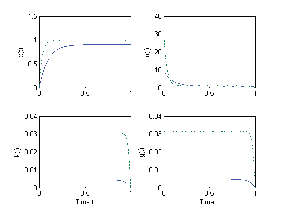
To illustrate the optimal control of biproper systems, a scalar example is considered.
x The optimal control law and the closed loop system are, In Figure 1, optimal trajectories for biproper (solid lines) and strictly proper (dotted lines) are compared. The presence of control input at the output node with a non-zero value for d introduces a steady state error in biproper systems. Further the rise time and settling time for strictly proper system is much faster than the biproper system. The control input and the solution to the Riccati differential equation are also plotted in Figure 1.

| Minimize ( , ) J x u | (1) | |||||
| u | ||||||
| subject to the following constraints, | ||||||
| ( ) x t Ax t Bu t Ew t ( ) ( ) ( ) | (2) | |||||
| ( ) y t Cx t Du t Fw t ( ) ( ) ( ) | (3) | |||||
| The state, input and output vectors are represented by | n x R , | m u R and | r y R , respectively. The | |||
| disturbance input vector is given by | ||||||
| T | ||||||
| J | ( ), ( ) e T Qe T | { ( ), ( ) e t Qe t | ( ), ( ) } u t Ru t dt | (4) | ||
| t | 0 | |||||
| Where, | 1 2 , v v | is the inner product for the compatible vectors 1 v and 2 v . The error vector is | ||||
| ( ) ( ) ( ) e t z t y t | ||||||